Everything that we can achieve by using „standard“ Excel, can be achieved by using VBA.
One of these things is certainly Conditional Formatting. We already showed multiple ways and rules on which Conditional Formatting can be conducted, and in the example below, we will show how to set the highlighting rules through VBA.
Change Cell Color Based on Value with VBA
Just like for the standard Conditional Formatting, there are multiple ways to get to our solution using VBA. For our example, we will use the following table:
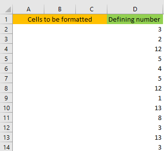
The goal is to highlight cells in column A to column C based on the value in column D. We will define the following rules:
- If the value in a cell in column D is from 1 to 5, then we want adjacent cells in columns A to C to be red.
- If the value in a cell in column D is from 5 to 10, then we want adjacent cells in columns A to C to be blue.
- If the value in a cell in column D is from 10 to 15, then we want adjacent cells in columns A to C to be yellow.
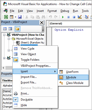
To define all of this, we will open up our Module by clicking on ALT + F11. After that, we will right-click anywhere on the left window and go Insert >> Module:
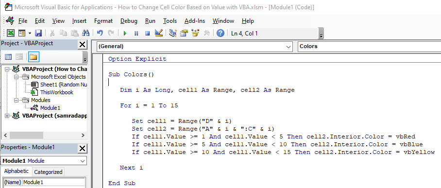
On the window that appears on our right side, we will insert the following code:
|
1 2 3 4 5 6 7 8 9 10 |
Sub Colors() Dim i As Long, cell1 As Range, cell2 As Range For i = 1 To 15 Set cell1 = Range("D" & i) Set cell2 = Range("A" & i & ":C" & i) If cell1.Value >= 1 And cell1.Value < 5 Then cell2.Interior.Color = vbRed If cell1.Value >= 5 And cell1.Value < 10 Then cell2.Interior.Color = vbBlue If cell1.Value >= 10 And cell1.Value < 15 Then cell2.Interior.Color = vbYellow Next i End Sub |
Our code looks like this in the Module:
For the first part of our code, we define the variables and set them in our If function:
|
1 2 3 4 |
Dim i As Long, cell1 As Range, cell2 As Range For i = 1 To 15 Set cell1 = Range("D" & i) Set cell2 = Range("A" & i & ":C" & i) |
Our variable “i” will be defined as long (number), while variables „cell1“ and „cell2“ will be defined as a range.
We will then create For Next Loop that will define that for numbers 1 to 15 (stored in “i” variable) we set variable „cell1“ to be equal to column D and whatever row we are currently on (variable „i“) and variable „cell2“ to be equal to the range of cells in columns A to C in the active row.
For the next thing, we define our If function:
|
1 2 3 |
If cell1.Value >= 1 And cell1.Value < 5 Then cell2.Interior.Color = vbRed If cell1.Value >= 5 And cell1.Value < 10 Then cell2.Interior.Color = vbBlue If cell1.Value >= 10 And cell1.Value < 15 Then cell2.Interior.Color = vbYellow |
As seen, we define that if the value in our variable „cell1“ (a cell that is located in the D column) is between 1 and 5, adjacent cells in columns from A to C (defined in the variable „cell2“) are highlighted in red color.
We go on and define that if the value is from 5 to 10 in cell D, then cells in columns A to C will be blue.
For the last case, these cells will be yellow if the value in the cell in column D is from 10 to 15.
For the last part, we write down:
|
1 |
Next i |
This will make sure that our If formula is applied to rows ranging from 1 to 15.
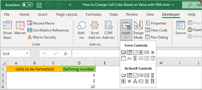
All we need to do now is make our code visible in our worksheet. To do so, we will go to the Developers tab >> Controls >> Insert >> Form Controls >> Button:
When we click on it, we will be presented with the option to create our button by drag and drop, and a window in which we can assign a macro will appear:
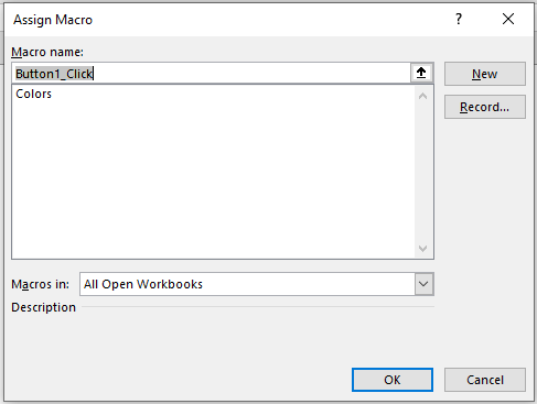
We will select the only existing Macro that we have- Colors, and then click on it and click OK. Once we do, we can change the name of our button, not to be a generic one (Button1), but to name it, for example, „Format Columns“:
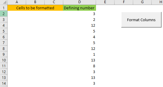
Now, when we click on it, our code will run and we will have the following results:
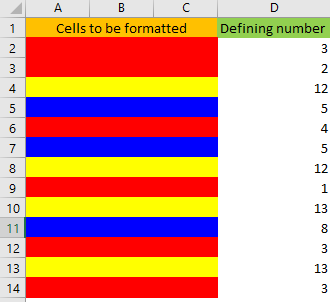
Which is exactly what we have defined in our code.