Use Index Match in Multiple Sheets in Excel

INDEX and MATCH are two functions that are most often used together. They are far superior that the VLOOKUP function which is maybe even more used.

In the example below, we will show how to use INDEX and MATCH in multiple sheets.

Quick recap

The Excel INDEX function is used to return the value of a cell at a given position in a range or array.

The syntax of this function is as follows:

Arguments are:

array – It can be a range of cells, tables, text, or anything where our values are found.

row_num – This represents a row position in the defined array.

col_num – [optional] This represents a column option in the defined array.

area_num – [optional] Here we input the range in reference that we should use.

The MATCH function is used to search a specified item in a range and then to return the relative position of that item in the range.

Its syntax is:

Arguments are as follows:

lookup_value: This is a required field. Here we input the value that we want to find in lookup_array.

lookup_array: Also required. We declare the range where our value is located.

match_type: This is an optional field that can have three values: -1, 0, or 1. This argument defines how Excel matches lookup_value with values in lookup_array. Value 0 represents the exact value of the lookup_value, and we will use this one.

Index and Match from Another Sheet

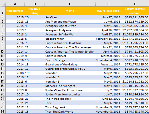
For our example, we will use the list of all Marvel movies, along with their respectful revenue rating (in comparison with the other Marvel movies on a list), release year, release date in the US, and box office gross revenue. We will put this table into a sheet called “Marvel movies”.

To create the Index and Match table, we will first create another sheet and call it simply „Index & Match“.

In that sheet, values in column A will be as follows (these are the values that can be found in the first row of our original table):

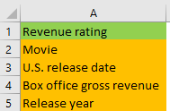
Revenue rating will be our lookup value for row_num (this value will be in cell B1), while other values in column A will be our lookup values for column_num of our INDEX function.

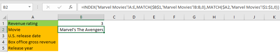
Having that in mind, we will randomly put the number 3 in cell B1.

In cell B2 we will input the formula as follows:

We will explain the formula in detail below:

First, we start by entering our INDEX formula.

The first argument that we have to enter into the formula is an array. Since we will be needing data from the whole table, our array will be every cell in a range from column A to column E.

So, our array is ‘Marvel Movies’!A:E (In the first part of the string we are referencing the sheet with the data. That is why we have apostrophes surrounding the name of our sheet. We have “!” as well since that is also an obligatory part when referencing another sheet. Finally, we added the columns).

Next, we need to define row_num, i.e. we have to find the position of our desired cell in rows. That is where the MATCH function comes into the picture. We enter it and we type in our desired lookup_value (cell B1). We lock this cell, as we want to use this cell’s reference for searching different values.

Then we define lookup_array (where this value could be located in our table. We know it is column B, so we reference the whole column in the “Marvel Movies” sheet, and match_type (0 for searching exact value).

Finally, we have to define the column_row. The reference cell is cell A2. We will only lock the column for this cell, so it will always be column A, but the rows can be changed. Our lookup_array is found in the “Marvel Movies” sheet again, and the value is located in the first row, hence the syntax: ‘Marvel Movies’!$1:$1.

We also need to lock these cells as well, as all of our values located in column A in this sheet are located in the first row in sheet “Marvel Movies”. Our match_type is again 0.

The result of our formula is as follows:

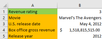
With this formula and defined cells in this way, as well as locked cells and the order of the columns in the first column, we can simply just copy and paste our formula to the cells in the B column (from B2 to B5).

When we do that, we will have all of our data populated:

The formula in cell B3 is as follows:

We can see that, in comparison with the first formula that we explained, the only difference is that we now have cell A3 instead of cell A2 as the lookup_value in the second MATCH formula, which defines the column_num for our INDEX formula.

We could have used only the data from the table. We will do that for the release year. The formula looks like this:

As seen, for the INDEX array Table1[#All] is used. Table1 is the name of our table, and „All“ stands for all the data.

Lookup_array for the first MATCH function is Table1[[#All],[Revenue rating]], i.e the column where revenue rating is located.

Lookup_array for the second MATCH function is the Headers from our table, which is the first row.

If we would add a row or a column to our table, this row or column would become an integral part of the table and we could apply an existing formula to find the desired value.