Excel: differences Between SUMPRODUCT, SUMIF, and SUMIFS

If you had an encounter with Excel in the past, you must have used some of the basic formulas that Excel has: SUM, MIN, MAX, or similar.

There are, of course, more complicated functions than these basic ones, but there are also combinations of basic function SUM and various criteria. We will present these in the text below.

Sumif Function in Excel

SUMIF function is simple to explain. It returns the sum of cells if they satisfy a certain condition. Criteria can be anything you define.

This function has three parameters:

• Range– required. In this part, we define the range that we want to be evaluated.
• Criteria– required. Anything we want to be our reference, be it text, number, or dates.
• Sum_range– Optional.

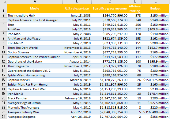
As in previous examples, we will use the table of Marvel movies with the release date, gross revenue, all-time ranking by revenue, and budget for our explanations.

We already said that criteria can be in a form of text. So we will sum the box office gross revenue of three Iron Man movies in the table above. For this example, we will need to populate all three of the parameters of the SUMIF function.

In cell C25 we will input the following function:

Our range, where our criteria are found, is located in column A (the list of movies).

Since we want to include all of the Iron Man movies, we will insert an asterisk before and after our desired word. The asterisk is normally a wildcard. In Excel, it replaces any number or character.

Finally, our sum_range is located in the C column, where gross revenue is found. 

Our final result will be the sum of gross revenues of Iron Man movies, part number 1, 2, and 3: 

Sumifs Function in Excel

The SUMIFS function is the same as SUMIF. The only difference is that, for this function to work, it has to comply with multiple criteria, not just one, as in SUMIF.

It has the following parameters:

• Sum_range (required). The range of cells to sum.
• Criteria_range1 (required). The range that is tested using Criteria1.

Criteria_range1 and Criteria1 work together. We have to define the criteria and range in which these criteria are to be found. Once these items are found, their corresponding values in Sum_range are added.

• Criteria1 (required). The criteria that define which cells in Criteria_range1 will be added.
• Criteria_range2, criteria2, … (optional)

In our case, we will sum the revenues of all the movies that are in the top 100 in terms of all-time ranking and that have the word „Avengers“ in their name.

We will put our formula in a cell C26 and the formula will be:

First, we define our sum_range. This is the range from which we will derive our final numbers. Since we want to find out the revenues of these movies, we will select the range C2:C24 as sum_range. 

Next, we have to define the cells in which our first criterion is located. Our first criteria are that the movie is in the top 100 movies all time ranked. For this criterion, the range is D2:D24. Our criteria are „<100“, so we added that in the next step. Notice that we had to put our criteria in quotation marks for the formula to work. 

For our second criterion (movies that have the word Avengers in their name) the range is column A (range A2:A24 to be exact) and our criteria is the word Avengers in quotation marks and with an asterisk so that we make sure to include all of Avengers movies.  

Sumproduct Function in Excel

As a final formula that we can use to calculate the budget of our movies based on certain criteria, we will present the SUMPRODUCT function.

The SUMPRODUCT function multiplies the range of cells or arrays and returns the sum of products. It first multiplies and then adds the values of the input arrays.

This function is very similar to SUMIFS, but it is more mathematical calculation-based while SUMIFS is more logic-based. You can use SUMPRODUCT to find the sum of products as well as conditional sums. SUMIFS cannot be used to find the sum of products.

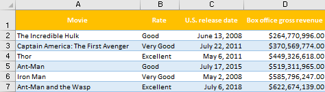
For our example, we have added one more column to the table. The column name is Rate, and it has three values: Good, Very Good, and Excellent. We placed these values in the B column. These data are completely random and are used for example purposes only.

We want to find out the total revenues of all „Excellent“ movies. As already mentioned, SUMPRODUCT works with arrays, and has arguments as follows:

• array1 – The first array or range to multiply, then add.
• array2 – optional. The second array or range to multiply, then add.

The purpose of the SUMPRODUCT function is to multiply, then sum, arrays. If only one array is supplied, SUMPRODUCT will simply sum the items in the array. Up to 30 arrays can be supplied.

So, to create our formula, we will define arrays and formula in cell D27 as follows:

The double-negative in the formula is used to convert TRUE and FALSE values into 1’s and 0’s. It tells Excel if the values in the array are true to the criteria („Excellent“) or not.

Our first array is column B (range B2:B24). Excel goes through all of these cells and checks if they satisfy our desired criteria. Double negative helps convert these values into binary numbers, and return 1 if true, and 0 if false.

So, for our first three rows, we will have:

• B2 = Good = False. Will return 0.
• B3 = Very Good = False. Will return 0.
• B4 = Excellent = True. Will return 1.

Each item in the first array (B2:B24) will be multiplied by the corresponding item in the second array (D2:D24).

So, the first number that we will have will be a product of cell B4 (value=1) and cell D4 ($449,326,618).

We can show our first three rows in curly-brace syntax as well:

So basically, what our function did is that it first looked in the first array (B2:B24) found all the „Excellent“ values, and turned them into binary values of 0 or 1 (1 if is Excellent, 0 if not) with the help of double negative, then looked in our second array (D2:D24) and multiplied the values in this array with corresponding values in the first array.

Finally, all of these products that we got in the first step were summed to get our final number:

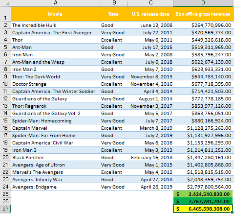
Since most of the values in the first array will return as 0 values, we will only have the values in those rows that return the value 1 in range B2:B24. Those will be the rows with „Excellent“ values in column B: 4, 7, 10, 13, 16, 19, and 22.