Not very often can happen that we need to return the actual reference of a certain cell, instead of the cell value itself. If, however, you happen to need this information, we will explain how to do this in the example below.
Return Cell Reference Instead of Value
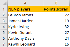
For the example, we will use the list of NBA players and points scored in one random night:
Now, let us presume that we want to find out in which exact cell LeBron James is located. For the following formula to work, we will presume that we already know the column number of the thing that we are looking for. We will enter the name of LeBron James in cell E2, and the following formula in cell F2:
|
1 |
=ADDRESS(MATCH($E$2,$A$1:$A$7,0),1) |
This formula is fairly easy. First, we input ADDRESS, which is a basic formula to return the cell reference. To make this formula work, we have to provide row and column numbers, in that order. For row, we use the MATCH formula to match the exact name of Lebron James located in cell E2 with the cell where this value is found in range A1:A7.
We then use the number 1 as a column number, as we said that is a constant. We get the following results:
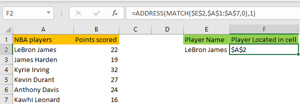
Now, this is the exact figure that we need. If we would change our constant, i.e. our column number to be any other number, for example, number 3, we would get an incorrect result:
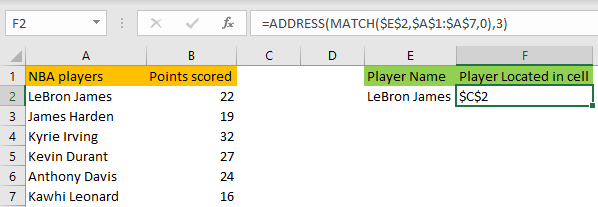
We still get the right number for rows, which is something. However, we need a little tweak to make this formula work for both rows and columns.
To do this, we will input the following formula in cell F3 (we placed desired player- Kyrie Irving in cell E3):
|
1 |
=CELL("address",INDEX(A1:B7, MATCH(E3,A1:A7,0),0)) |
The CELL function returns us information about the formatting, color, type, etc. of a specific cell. The list (not full) of options that we can use is as follows:
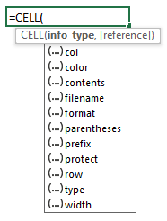
We will choose an option that is not presented in a list, which is “address”. After that, for a reference of our cell, we will use INDEX and MATCH. Our array for the INDEX formula will be columns A and B. For the rows, we will use MATCH to find the value of our cell in the range A1:A7. For columns, we input just the number 0.
This is the result we end up with:
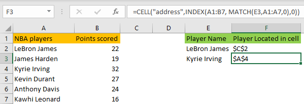
We get the result that shows cell A4, which is the exact cell where Kyrie Irving is located in our table.