How to Lookup the Nth Value in Excel

So far, we showed and you are probably aware of the two cool functions- VLOOKUP and INDEX (in a combination with the MATCH function) that are used as lookup options in Excel.

However, these functions are only used for the first instance of the lookup value. But what if we want to find the second, third, or any other lookup value?

For these cases, we need to use other functions and formulas. We will show two ways to do this in the examples below.

Lookup the Nth Value Using Another Column

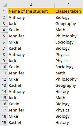
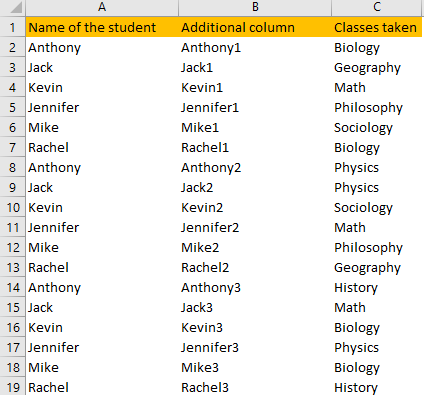
For our example, we will use the list of students’ names and the classes that they are taking:

First thing first, if you want to find the unique names in our first column, you can use the UNIQUE function:

As in the picture below:

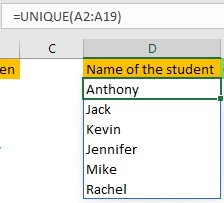
The UNIQUE function recognizes unique values in an array and returns them. It is an array function added to the Office 365 version of Excel.

We will add columns for classes next to column D, and will use a VLOOKUP formula to see if we will get the needed results:

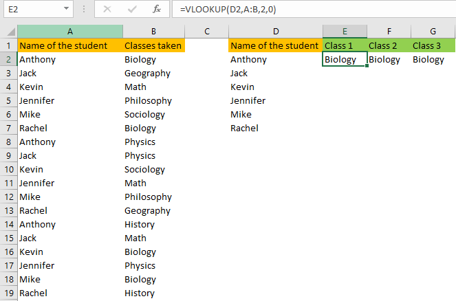
Of course, the VLOOKUP function always returns the first value, i.e. Biology for Anthony.

To change this, we will add a column between column A and column B, and we will insert the following formula:

We will drag this formula till the end of our table, and we will have the following results:

The COUNTIF formula in column B adds a number to the name of every employee to make it unique. First Jack that it finds becomes Jack1, the second becomes Jack2, and so on.

Now we have unique values that are related to values in column A.

To find the classes for every student, we need to add the following formula in cell F2 (the first cell in which we want to find the class):

We will input this formula into our table, and have the following results:

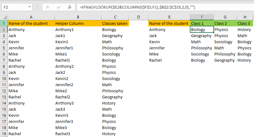
What changed for this VLOOKUP? Well, now it has unique names that can help out when finding the matching course.

Our lookup value is $E2&COLUMNS($F$1:F1). It adds the number to the employee name based on the number of the column. When we use this formula for Kevin (cell F4) the lookup value is “Kevin1”. The next lookup value in the same row will be “Kevin2” and so on.

Lookup the Nth Value Using Array Formula

If you do not want to be in a situation to add a new column all the time, you can use a different approach. We will copy and paste the original table to the new sheet. We will not, however, add another column.

The whole preparation for the new formula looks like this:

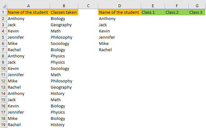
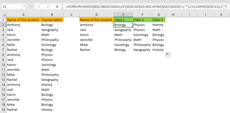
In cell E2 we will input the following formula:

The above is the array formula. If you are using an older version of Excel, to make this formula work you need to insert it with the combination of CTRL + SHIFT + ENTER. Simple ENTER will not do the trick.

However, array formulas are integrated into new Excel versions (2019 and Office 365) so if you are working in these environments, you will not need the above-stated combination. Input ENTER and go for it.

So how does exactly the above formula work?

The first important part of the formula is:

This part observes every cell in range A2:A19 with the value in cell D2. The value in cell D2 is “Anthony” so this formula checks if this value is found in the range A2:A19 or not.

It goes through every cell in this range and returns TRUE and FALSE values.

For the next part, we have:

This formula uses the TRUE and FALSE values that we found above and replaces the TRUE value with the position of this value in our range, and FALSE with blanks.

Then we have the SMALL function in our formula:

This formula picks the smallest numbers from our array. It uses the COLUMN function to successfully show column numbers.

Now we add the INDEX formula to the mix. This function returns a value from column B having in mind the position that is returned by the SMALL function. In cell E2, it will return „Biology“, as it Is the first item found in range B2:B19. Then, in cell F2, it will find „Physics“, and so on.

With everything said above, our table looks like this: