When we use the IF function for whatever reason, we need to have certain criteria that have to be met in order for our function to retrieve a proper value.
These criteria can be anything in our data.
Find a Value in a List with an If Function
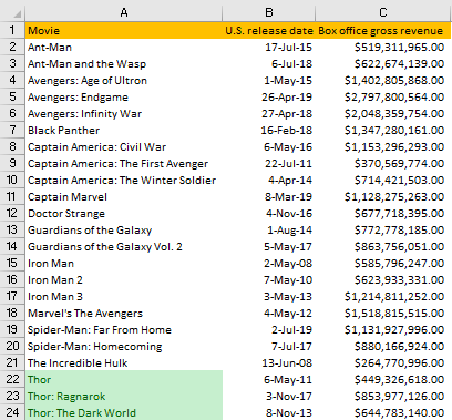
There is one formula that can help us with finding a certain value in our list. For example, let us say we have a list of all the Marvel movies. Now, we want to make sure that the Thor movie is on this list.
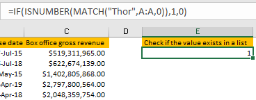
To do this, we will put a value: „Check if the value exists in a list“ in cell E2 and we will input the following function in the E2 cell:
|
1 |
=IF(ISNUMBER(MATCH("Thor",A:A,0)),1,0) |
Our logical test for this IF function first checks if our value is equal to the „Thor“ value (lookup_value of our MATCH function). If it is, Excel will return value 1. If not, it will return the value 0.
We will have a value of 1 returned since we have a Thor movie on our list.
Get Results If Value Is in the List
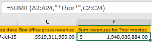
If we know what value we are searching for, we can combine various functions with our condition. For example, we can use the SUMIF function to find out the total revenues of Thor movies.
As we can see, we have a total of three Thor movies on our list. To sum all the revenues from these movies, we will input the following formula in cell F2:
|
1 |
=SUMIF(A2:A24,"*Thor*",C2:C24) |
The SUMIF function returns the sum of cells in a range that meet a single condition.
We have three parameters for this function:
- Range. Here, we type in the range from which we are searching for our condition. In our case, the range is A2:A24.
- Criteria. Our criteria are Thor movies. We want to include them all and we use “*” to make sure to include all the movies that contain this value, regardless of the text in front or after this value.
- Sum_range. In our final step, we have to specify what are the values that we want to sum. For us, these values are found in column C and we will input the range C2:C24.
Our final result will be just a little less than $2 billion.
Formatting If a Certain Value Is in a List
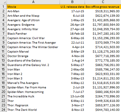
There is also an easy way for us to highlight all the values in our list that have a certain value. We will use Thor movies again for our example.
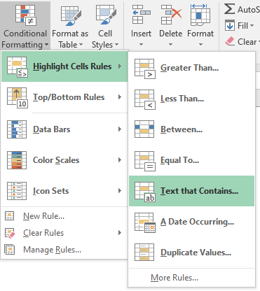
To do this, we have to select column A and go to Home >> Styles >> Conditional Formatting.
In the Conditional Formatting dropdown menu, we select Highlight Cells Rules and finally Text that Contains.
Once we do all of this, we have to input Thor movie to clarify what we want to be highlighted.
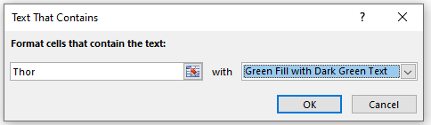
We will choose green fill with dark green text, and we will see the changes in our table immediately. We click OK and have the result as follows: