We have all been in a situation where we realize that we have made the same error in a whole document, or a whole worksheet, which can be easily resolved if we just replace some certain value with another one.
For these instances and occurrences, we can use the Find and Replace option in Excel.
Using Find and Replace
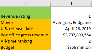
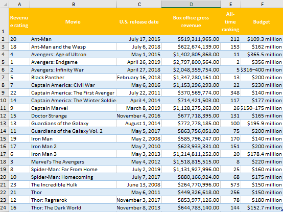
For our example, we will use the table that we created for explaining the functionalities and use of the Index and Match functions. The table presents the list of all Marvel movies with their revenue rating (in relation to other Marvel movies on the list), release date, gross revenue, all-time ranking, and budget.
In relation to this table, we have also created the Index and Match functions that can help us easily navigate and find the movie based on their revenue rating. For our function to work and values to change, we only have to change the value in cell I2 i.e. revenue rating.
Let us now assume that we want to find the first part of the Thor movie and replace its name with Thor: Original one.
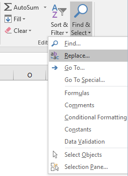
For this, we can either click on CTRL + H or go to the Home tab, find the Editing subtab, go to Find & Select, and then choose Replace from the dropdown menu.
We will then type our desired data into the Find what: and Replace with: fields in the pop-up window and then click on Find Next .
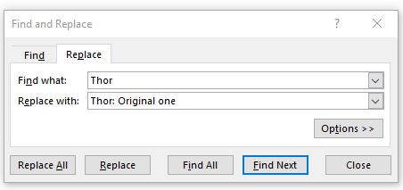
The movie called Thor is the first one inside our table so when we find it we will just click Replace and then close our Find and Replace window.
We do not want to click on Replace All, since we would replace the values in all three of the Thor movies.
Find and Replace in Formulas
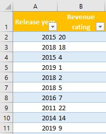
Now, let us assume that one thing occurred. We created another column at the beginning of our worksheet, and we named it Release year. This is now column A. Moreover, we have copied and pasted data from previous column A to column B.
So basically, now column B is the Revenue rating column.
To find out the release year of the movies, we will use the formula:
|
1 |
=YEAR(serial_number) |
In our case, the serial number is the U.S. release date, so our A2 row will have the following value:
|
1 |
=YEAR([@[U.S. release date]]) |
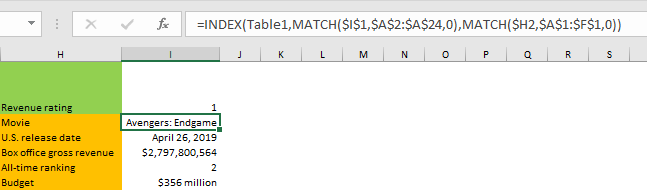
One thing that happened since we changed the data in our A column. Now, our Index and Match formulas simply do not work, and they show #N/A (not applicable, not available) data:
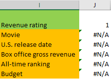
Our formula in cell J2, which is the cell right to the Movie text in the picture below is:
|
1 |
=INDEX(Table1,MATCH($J$1,$A$2:$A$24,0),MATCH($I2,$A$1:$G$1,0)) |
From the look of this formula, we have to change the value of lookup_array in our first MATCH function that defines our row_num values.
We will not have to do anything with the second MATCH function, which defines column_num since it was not impacted by the changes.
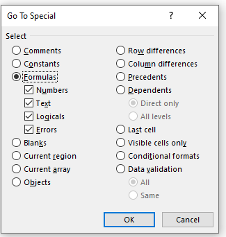
Since we want to change only the number in our formulas, the good thing for us is to select the range or the worksheet we are using, press Ctrl + G to enable Go To dialog, and then click Special.
We can also find Go To dialog in the same location as we did for Replace, and that is Home >> Editing– Find & Select.
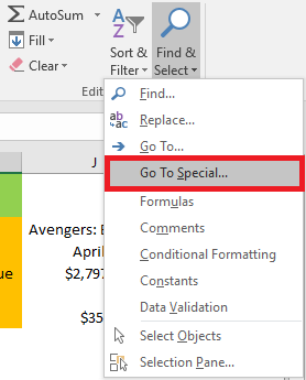
Once we get to this option, we will click on Formulas so that we select only the cells with formulas in our worksheet.
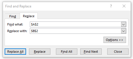
We click OK and then click again on CTRL + H to get to Find and Replace. We will find all of the $A$2 values and replace them with $B$2. To do this, we input the values into Find what: and Replace with: fields and then click Replace All.
Excel will inform us about the changes made:
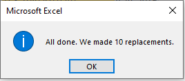
We will then click OK to see the changes.
Our table looks normal again: