We have already shown various benefits of conditional formatting and its uses. However, it was not shown how to use this useful functionality when we have blank cells in our table.
We will show how to use this in the example below.
Conditional Formatting of Blank Cells with Rule
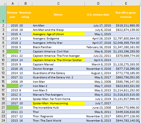
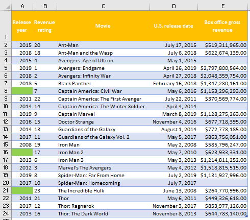
For our example, we will use the list of all Marvel movies that were released until the end of 2019 with their release year, revenue rating (compared to each other), titles, U.S. release date, and box office gross revenue.
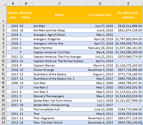
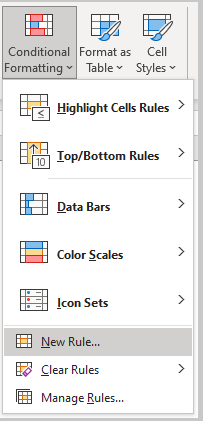
We can see that we lack certain years in the first column and certain box office revenues figures. We want to highlight all the rows in the first column where years are missing. To do so, we will select our range (A2:A24) go to the Home tab >> Styles >> Conditional Formatting >> New Rule:
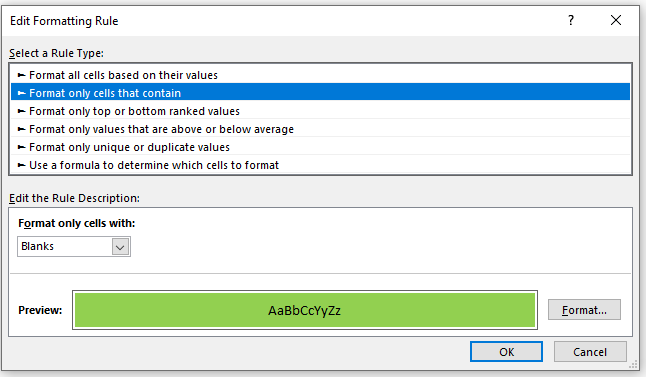
On a pop-up window that appears, we will choose Format only cells that contain, and will choose “Blanks” on Format only cells with dropdown. We will then click Format and choose any color in the Fil tab (in our case it will be green). Our pop-up window will look like this:
When we click OK, our table will look like this:
Conditional Formatting of Blank Cells with Formula
There is also a formula that we could use to get the same results. That formula is ISBLANK. This formula checks desired cell or range and returns the value TRUE if it is empty, and FALSE if it is not.
We want to highlight the names of the movies for which we lack box office revenue gross. We will select the range C2:C24 and follow the same steps as in the first example (Home tab >> Styles >> Conditional Formatting >> New Rule).
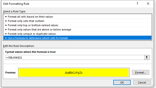
On the pop-up window that appears, this time we will choose another option- Use a formula to determine which cells to format, and we will input the following formula:
|
1 |
=ISBLANK(E2) |
We will choose these cells that are found to be filled in yellow color:
When we click OK now, we will notice that rows 4, 10, and 20 are the ones populated with yellow color in column C, and those are the ones that do not have values in column E: