Use Conditional Formatting to Compare Lists in Excel

We have proven the usefulness of conditional formatting in Excel on multiple examples.

We will show another cool feature in the example below, which will refer to the comparison of two lists with conditional formatting.

Using Conditional Formatting to Compare Lists

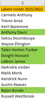
For our example, we will use the list of NBA players that played for the Los Angeles Lakers in the 2020/2021 season and the ones that will play in the upcoming season (2021/2022).

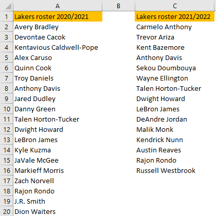
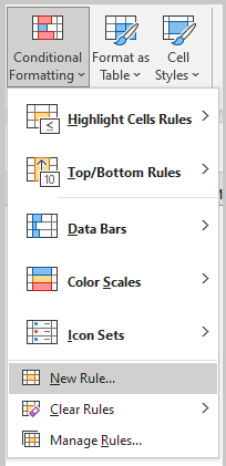
If we want to highlight only those players that are on the roster for the upcoming season and who were a part of the team a year before, we need to select the desired range (C2:C16) go to Home tab >> Conditional Formatting >> New Rule:

To achieve what we want, we must follow the following formula:

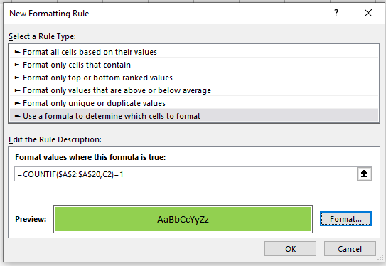
So, on the pop-up window that appears, we will select the last option, which is: Use a formula to determine which cells to format, and input the following formula:

We will then define that the cells with these cells are filled with the green color:

How does this formula work? COUNTIF function will check if the value in our cell C2 can be found in the range that we used for comparison (A2:A20). If this value is found, our formula will return a 1, meaning that our conditional formatting will be triggered.

We are locking our range, as it is always the same, but we do not lock the first value, to encapsulate every cell in the second range.

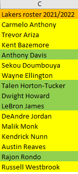
Finally, we will click OK, and have the following results:

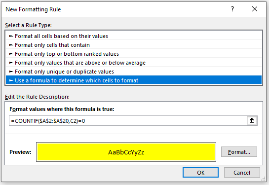
If we wanted to highlight those players that are new additions to the team, we would have to use the following formula:

We will repeat our steps with this formula as the new rule, and set these players to be highlighted in yellow:

When we click OK, our table will look like this: