We have already shown the usefulness of conditional formatting and the various occasions on which it can be used.
In the example below, we will show how to use conditional formatting with the average formula.
Combining Average and Conditional Formatting
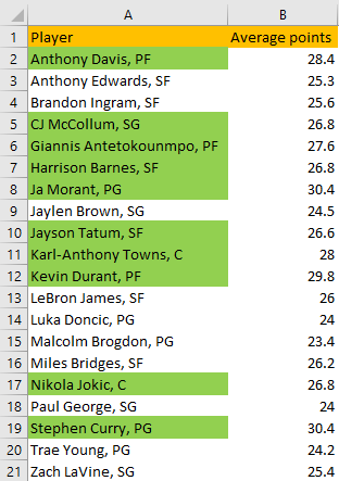
We will show above stated with the table of the best NBA scorers in the season 2021/2022 so far:
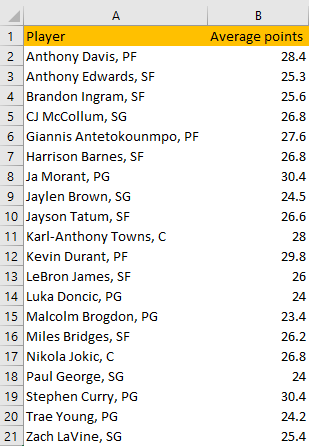
Now we want to highlight only those players in column A that have more points than the average of all the players in the table.
We can do this in two ways- we can directly input the formula in Conditional Formatting or place the formula in the sheet and then use Conditional Formatting:
- Formula directly in Conditional Formatting:
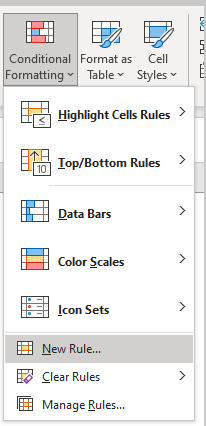
To do this, we will select range A2:A21 and then go to Home >> Conditional Formatting >> New Rule:
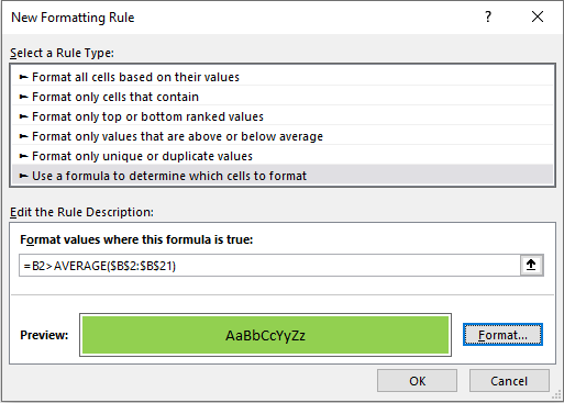
On a pop-up window that appears we will choose the last option- Use a formula to determine which cells to format, and we will input the following formula beneath the line: Format value where this formula is true:
|
1 |
=B2>AVERAGE($B$2:$B$21) |
We will format all of these cells in column A with green color. The pop-up window will look like this:
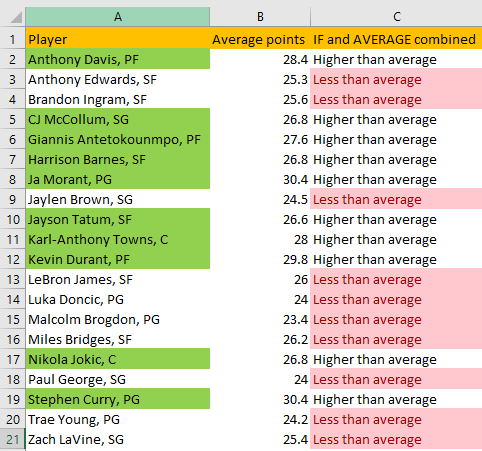
Once we click OK, our table will look like this:
- The formula in the sheet directly
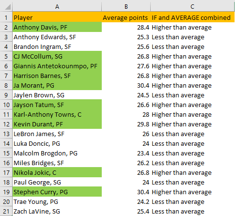
We can also combine the IF and AVERAGE formulas on our sheet directly and then use the results that we get to highlight the players.
We will put the formula in column C, and it will be like this:
|
1 |
=IF(B2<AVERAGE($B$2:$B$21), "Less than average", "Higher than average") |
What this formula does is that it checks if the number in cell B2 is smaller than the average in the range B2:B21 (these cells are locked as the range will not change) and gives out the result “less than average” if the statement is true and “higher than average” if this statement is false.
We will drag this formula to cell C21. Our table looks like this:
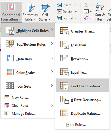
Let us say that we want to find all the players that have fewer points than the average. To do this, we will select range C2:C21 and then go to Home >> Conditional Formatting >> Highlight Cells Rules >> Text that Contains:
When a pop-up appears, we will input any word from column C that is specific so that we can find players with fewer points than average. We will simply input the word “less” (it can be the lower case as well):
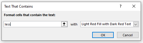
When we click OK, cells in column C with players that have less than average points will be highlighted in red color: