Pivot Tables are among the best ways in which we can manage our data in Excel. They give us a great opportunity to manipulate the information that we have.
In the example below, we will show a couple of useful things when dealing with sorting the data in the Pivot Tables.
Creating and Making Pivot Table Neater
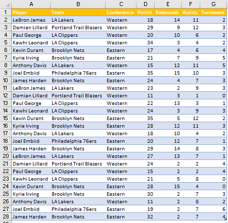
For our example, we will use the list of NBA players and their statistics for several categories and for several playing nights (three, to be exact):
Now we will create our Pivot Table by selecting the table and going to Insert >> Tables >> Pivot Tables. Once we click on it, a pop-up will appear:
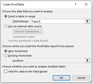
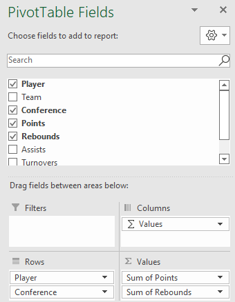
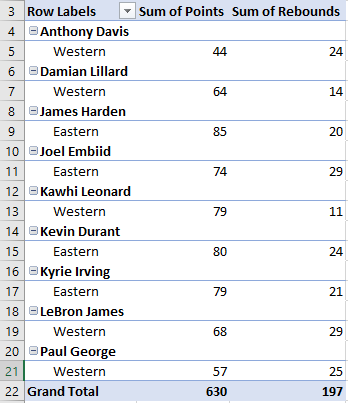
We will just click OK and Pivot Table will be created in a new sheet. We will name this sheet “Pivot Table” and add Player and Conference to Rows Field, and Points and Rebounds to Values Field:
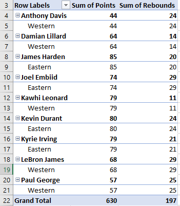
Our table looks like this:
To make our table a little neater, we will first click on it and then go to Design Tab >> Subtotals >> Do Not Show Subtotals:
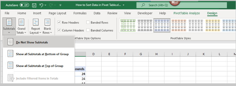
This will remove subtotals and clean our table a little bit:
Next thing, we will right-click anywhere on the table, and then go to the Display tab and choose Classic PivotTable layout:
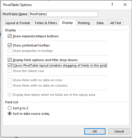
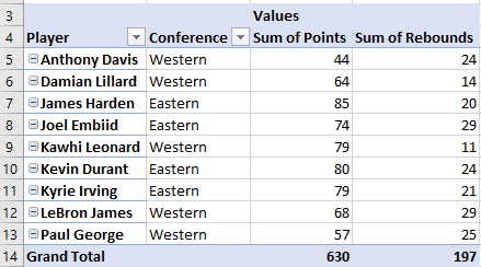
Once we do this, our Pivot Table will look way neater:
Sorting Data in Pivot Table
It is important to know that our data needs to be sorted in some way. As seen, in our case, the data is sorted out in alphabetical order. The row for which we can manipulate the sorting options is the first row in our table, i.e. Player, meaning that we can only use the dropdown in this row to sort the table.
We will click on a dropdown button of the first row and will notice that we have two generic sorting options (from A to Z and Z to A), that are given due to the fact that Excel recognizes the data in the first column as a string, which is the case.
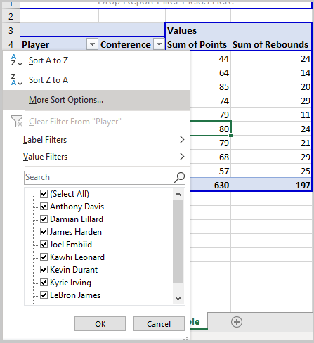
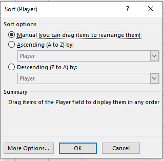
We will click on More Sort Options and the following window will appear:
Remove Sort from Pivot Table
You will see that the first option that you have at your disposal is Manual and the explanation is that you can simply drag items to rearrange them.
When you get back to the table, you will notice that you can select any cell in column A and drag and drop it anywhere you like:
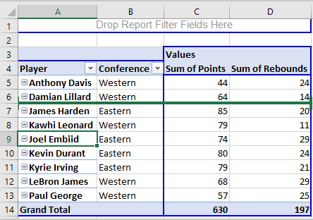
In our case we will move Joel Embiid to third place in the table (our data will be placed beneath the green line):
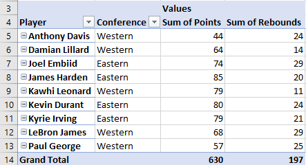
As this random placement of our rows makes sorting illogical, we can practically say that we removed sorting with this option.
When we get back to sorting options, you will notice that we can sort our data either by ascending or descending the columns Player, Sum of Points, and Sum of Rebounds.
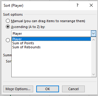
We cannot manipulate the second option in Rows Field, which is, in our case, Conference.
There are also more sorting options, and we can get to them by clicking More Options. Once we click on it, the following window will appear:
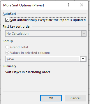
When we uncheck the button Sort automatically every time the report is updated, we will have option First key sort order available:
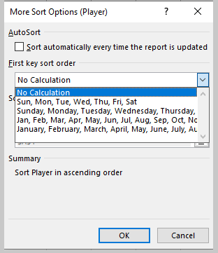
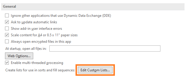
The options that we see in this dropdown are called Custom Lists. You can create your own Custom Lists by going to File >> Options >> Advanced and then scroll all the way to the bottom, go to General, and then click on Edit Custom Lists:
When we click on it, we will have the following options presented.
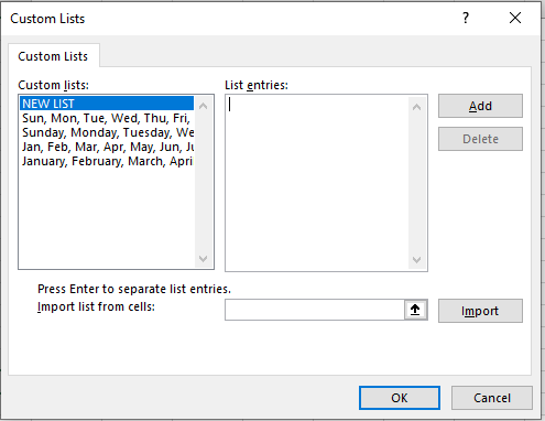
We can either add the list by writing basically whatever we want. We can also click on Import and choose the list from any worksheet in our workbook. Once we click OK, our list will be added, and we will have an option to choose it by repeating the steps above.