In Excel, there are usually multiple ways to do the same effect and achieve the same results. You can often choose the most convenient one, per your liking.
In the example below, we will show what options you have at your disposal for removing brackets and parentheses from your text in Excel.
Substitute Function
The first thing that we can do to remove brackets and parentheses is to use the SUBSTITUTE function. This one is pretty easy, and it has a few parameters: 1) we input the text that we want to change, 2) we input the old text, and 3) we input the new text.
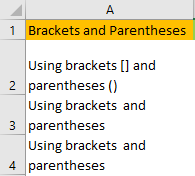
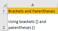
For our example, this is the original text:
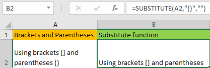
In the cell B2, we will place our SUBSTITUTE function:
|
1 |
=SUBSTITUTE(A2,"()","") |
This function will leave us without parentheses:
To remove the brackets that we have in our text in cell B2, we need another function. We will put it in cell C2:
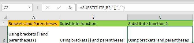
For the final result, it is noticeable that we do not have brackets not parentheses in our text. We are left with space in the text, however. We can use the same function to remove white spaces as well.
Find and Replace
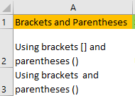
We can also use Find and Replace to remove brackets and parentheses. We will put our text (“Using brackets [] and parentheses ()”) in cell A4.
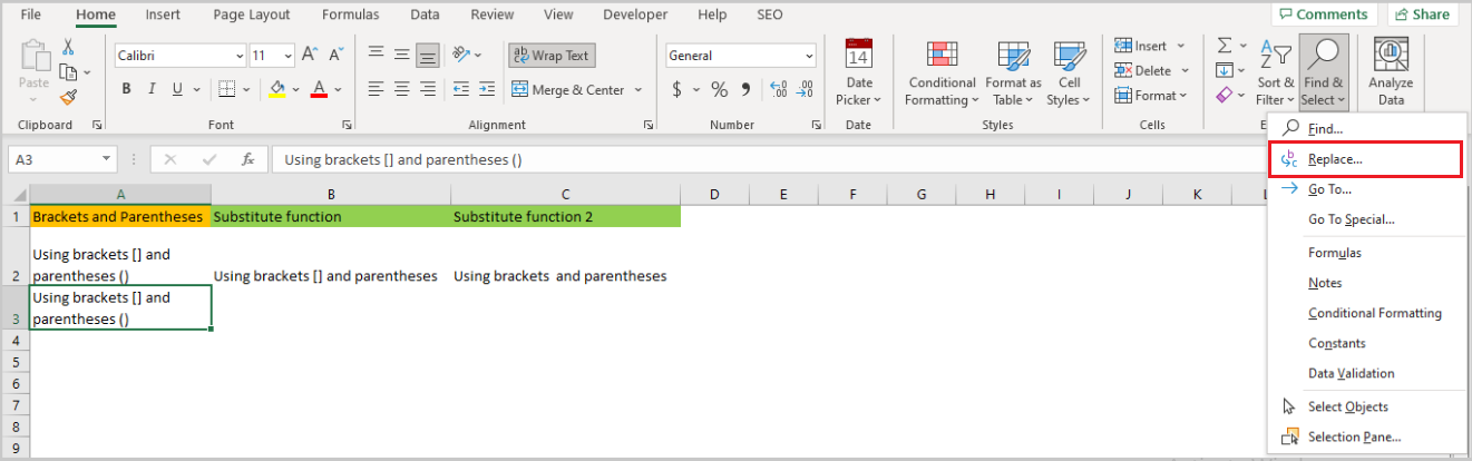
We will select this cell and then go to Home >> Editing >> Find & Replace >> Replace:
Or we can simply press CTRL + H on our keyboard to get to the same window.
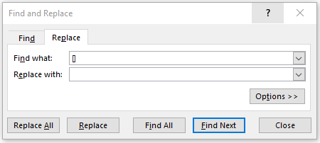
There, we will input [] in the Find what option. In Replace with we will simply leave blank. This is what the Replace window looks like in the worksheet:
When we click Replace, this is the text we will be left with:
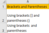
We will repeat the steps above to remove the parentheses, and finally, we will end up with this picture:
VBA
As always, we can also use VBA to achieve any goal we want in Excel. We will copy and paste the data from cell A2 to cell A4.
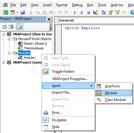
Next, we will open VBA by clicking ALT + F11 on our keyboard. On the window that appears, we will right-click on the left window, and then choose Insert >> Module:
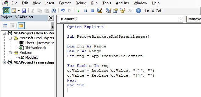
In the window on the right side, we will insert the following code:
|
1 2 3 4 5 6 7 8 |
Dim rng As Range Dim c As Range Set rng = Application.Selection For Each c In rng c.Value = Replace(c.Value, "()", "") c.Value = Replace(c.Value, "[]", "") Next End Sub |
This is what the code looks like in the module:
The first thing that code does is that it declares two variables- rng and c as a range. Then it sets our rng variable to be equal to the range that we selected.
For the last thing, we use For Next Loop to change the values for parentheses and brackets in every cell of our range (if there are multiple cells) with empty values.
This code is made in a way that the precondition is that we select the range that we want to change, and then we run the code. For our example, we will position ourselves and select cell A4. Then we will go to our module and click F5 on our keyboard to run our code.
This is the result we end up with: