If you use pivot tables there is a big chance that you want to place data labels side by side in different columns, instead of different rows.
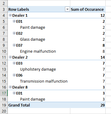
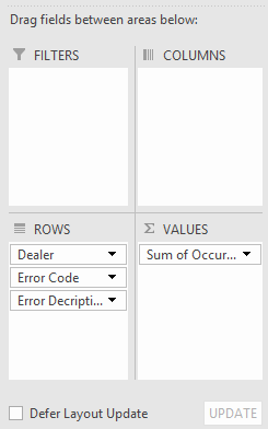
Normally when you create a pivot table, you get the following result.
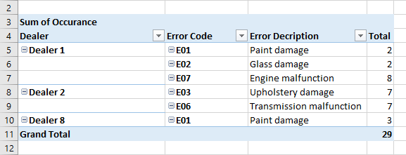
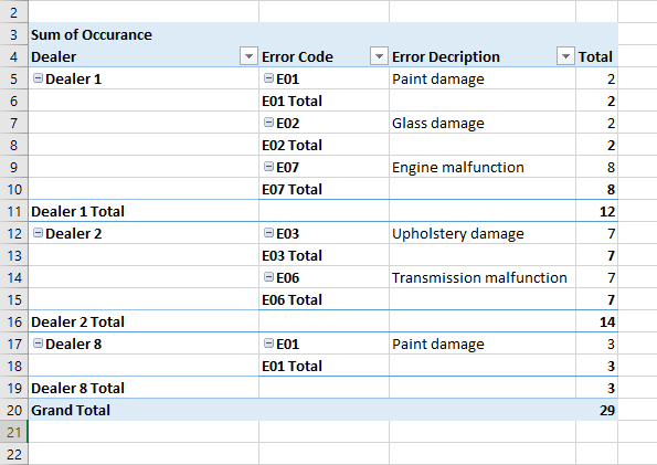
But this is not what we want. In this lesson, I’m going to show you how you can modify your pivot table to get the following result.
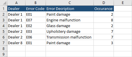
We are going to use the following example.
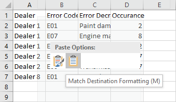
You can copy the following table and paste it into your worksheet as Match Destination Formatting.
| Dealer | Error Code | Error Description | Occurrence |
| Dealer 1 | E01 | Paint damage | 2 |
| Dealer 1 | E07 | Engine malfunction | 8 |
| Dealer 1 | E02 | Glass damage | 2 |
| Dealer 2 | E03 | Upholstery damage | 7 |
| Dealer 2 | E06 | Transmission malfunction | 7 |
| Dealer 8 | E01 | Paint damage | 3 |
Now, let’s create a pivot table (Insert >> Tables >> Pivot Table) and check all the values in Pivot Table Fields.
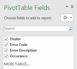
Fields should look like this.
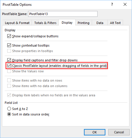
Right-click inside a pivot table and choose PivotTable Options….
Check the data as shown in the image below.
The table is going to change.
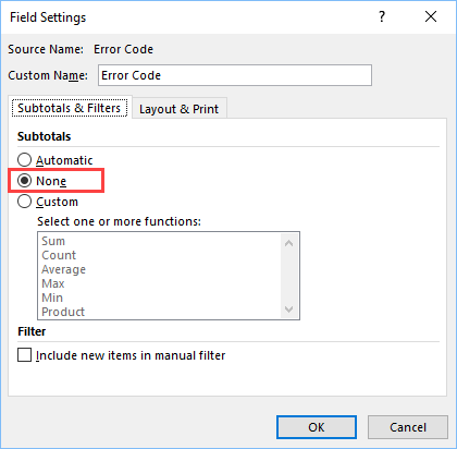
The pivot table is almost ready. What I don’t like are the totals inside Error Code and Dealer. We are going to remove them now.
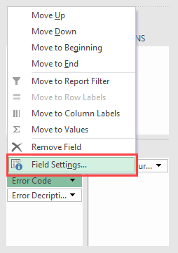
In order to do so, go to the field list click Error Code, and choose Field Settings….
Inside this window change Automatic to None.
Do the same to the Dealer field. Now, your table is ready.