In Excel, the default standard format displays negative percentage numbers with a “-” sign. When you are scanning a large Excel worksheet, it can be difficult to see these negative percentages that are displayed in the standard format. One way you can use to make them stand out so that you can easily locate them is by displaying them within parentheses.
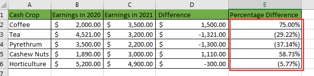
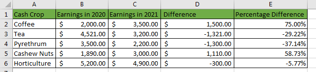
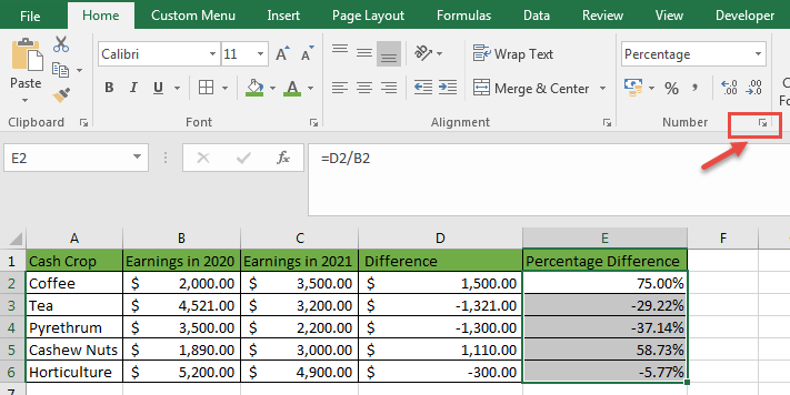
We will use the following dataset to demonstrate how to display negative percentages in parentheses:
How to Customise Numbers in Excel Using Codes
Excel does not come with a predefined format for displaying negative percentage values within brackets or parentheses.
To display the negative percentages in the dataset in parentheses, we must create a custom number format.
But before we can do it, it is important to know that Excel can return four different display formats for numbers. It has predefined parameters for positive values, negative values, zero, and text.
The parameters have to appear in the following order:
Positive value;Negative value;Zero;Text
To specify how a number should be displayed, use 0 to show a number or 0 if empty, and use # to display a number or nothing.
For example, if you have the number 456, the code #### will return 456. The code 0000 will display 0456, and the code ###0.00 will return 456.00.
Create Custom Code to Display Negative Percentages in Parentheses
With the understanding we have acquired so far concerning display codes in Excel, it is easy to construct a format for displaying negative percentages between parentheses.
For positive numbers use the code ###0.00, and for negative numbers between parentheses use the code (###0.00). To display positive percentages use the code ###0.00%, and to display negative percentages within parentheses use the code (###0.00%).
Follow the following steps to display the negative percentages between parentheses in our dataset:
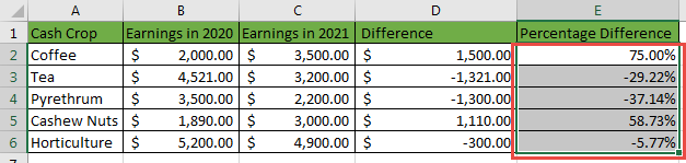
Step 1 – Select the cells in Column E that has the negative percentages that are displayed in Excel standard format that doesn’t support display within parentheses:
Step 2– Launch the Format Cells dialog box using the keyboard shortcut Ctrl + 1:
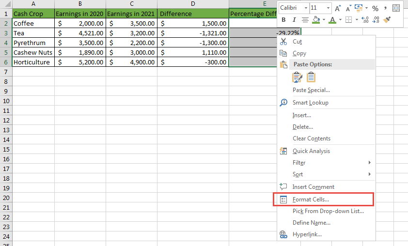
Alternatively, you can also open the Format Cells dialog box by right-clicking the selected cells in the dataset and clicking the Format Cells… command on the shortcut menu that pops up:
Another way to launch the Format Cells dialog box is by clicking the Number Format launcher button:
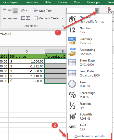
You can also open the Format Cells dialog box by clicking on the drop-down arrow on the Number Format drop-down box and then clicking the More Number Formats… command:
Once the Format Cells dialog box is open, proceed to the next step.
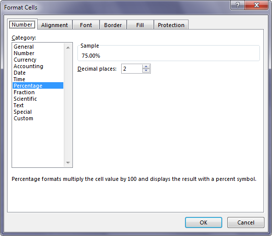
Step 3 – Select the Custom category at the bottom of the predefined formats in the Category box:
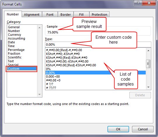
In the Custom category, you will see a list of code samples that you can use to display custom number formats and an area for manually entering codes in various combinations. You will also see an area for previewing sample results of the sample code you enter.
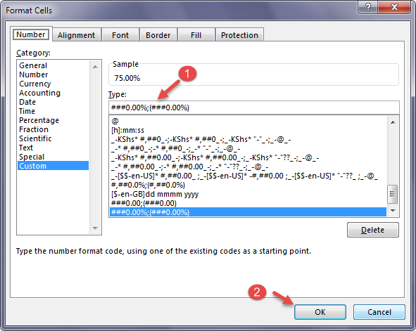
Step 4 – In the Type box enter the code ###0.00%;(###0.00%) and click the OK button to apply the custom code:
The result would be that the negative percentages will now be displayed between parentheses: