We have already explained how to number our rows in Excel in various ways, and how to format these numbers.
In the example below, we will show how to number the rows that are filtered in Excel.
Number the Filtered Rows
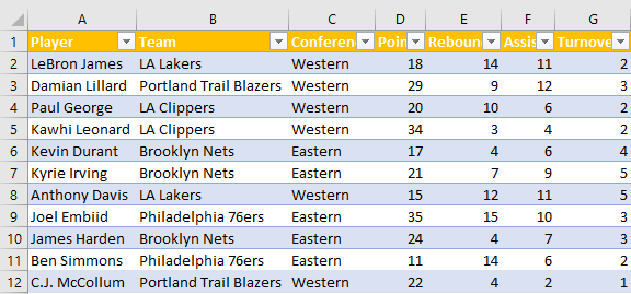
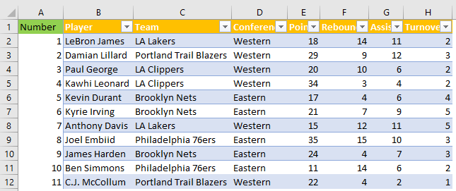
For our example, we will use the table with NBA players, and their statistics from several categories: points, rebounds, assists, and turnovers:
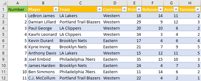
We will create another row that will be the new column A, and we will input the ordering numbers for our players:
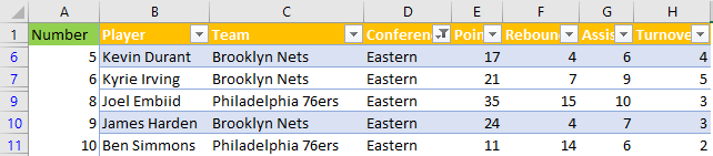
If we now filter only the players from the Eastern conference, we will notice that these numbers will not change, i.e. that we do not have the new order:
To make this work, we need to use the SUBTOTAL formula.
We will now remove the filter and delete the numbers in column A. In cell A2 we will input number 1 and in cell A3 we will input the following formula:
|
1 |
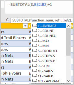
=SUBTOTAL(3,B$2:B2)+1 |
The SUBTOTAL function allows us to create groups and after that to perform various functions, such as SUM, COUNT, MAX, etc.
When we create it, we first need to choose the function (by the number) among many:
We will choose the COUNTA function for our needs. Then we need to define the reference cell. In our case, it will be the range that is the combination of the first cell in column B– cell B2, which will be locked, and cell B2 (which will be changed when dragged). We will then add the number 1 to this number.
Results in cell A3 will be number 2 (1+1), in cell A4 3 (1+2), etc.
We will drag this formula till the end of our list:
We will then filter only Eastern conferences in our table:
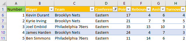
You can notice that although Kyrie Irving was numbered as player number 6 in the original table, he is now second on our list, and thus has the number 2 by his name.
This functions on a basis that the SUBTOTAL formula only observes the filtered data in our list, and it changed accordingly.