Insert a Tab Character in a Cell in Excel

In word-processing applications such as Microsoft Word, it is easy to insert Tabs. The tabs are used to align text by moving the cursor to a predefined position. One Tab is normally equivalent to five spaces. The purpose of Tabs is to increase the readability of a document.

In Excel, however, we cannot insert tabs in a cell but we may still want to improve the readability and visual appeal of our data by giving it a tabbed appearance.

How to achieve the appearance of tabbed information

Excel does not have an inbuilt way of inserting a tab in a cell. You can’t add a tab in a cell by simply pressing the Tab key on the keyboard as you would in a word processor. Pressing the Tab key in a cell simply moves the cell selector to the next cell on the right.

Although Excel does not have a way of inserting a tab character in a cell using the keyboard, sometimes in Excel you may want your data to be more visually appealing by having the appearance of tabbed information. This can only be achieved by using workarounds.

In this tutorial we will explore the following four workarounds that we can use to achieve the “tabbed appearance” in our Excel data:

1. Adding five spaces manually.
2. Use a combination of CONCATENATE, CHAR, and REPT functions.
3. Use CHAR function and code value 9.
4. Use the Increase Indent button.

Add five spaces manually

The easiest workaround to achieve the tabbed appearance in Excel cells is by adding five spaces manually at the beginning or within the text in a cell. We will need to add five spaces since one Tab is equivalent to five regular spaces.

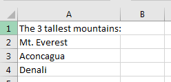
We will use the following data to show how this can be achieved:

We use the following steps:

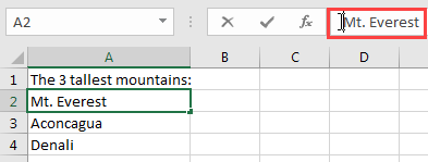
1. Select cell A2.
2. Move the cursor to the beginning of the text in the formula bar:

Alternatively, double-click in the cell and move the cursor to the beginning of the text, or press ley F2 on the keyboard and move the cursor to the beginning of the text.

3. Press the space bar on the keyboard five times to add five spaces to the beginning of the text:

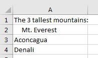
4. Repeat step 3 for cells A3 and A4:

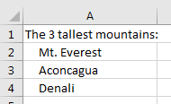
The dataset now has a tabbed appearance and improved readability.

Use a combination of CONCATENATE, CHAR, and REPT functions

The previous method of manually adding five spaces can be tedious and time-consuming.

This second method adds the five spaces using a formula by using the following steps:

1. Select cell B1.
2. Type in the formula:

and press Enter key.

Alternatively, we can simplify the formula by using the ampersand character (&) to join the character strings in the cells like:

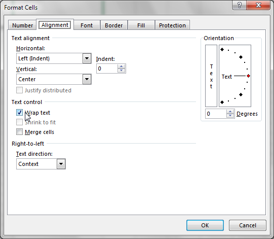
3. Press Ctrl + 1 on the keyboard to launch the Format Cells Dialog box. Under the Alignment tab check the “Wrap text” control and press OK:

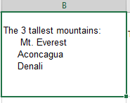
The data in cell B1 now has a tabbed appearance:

4. Select Cell B1 and press Ctrl + C on the keyboard to copy the data.
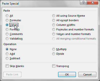
5. Select Cell C1 and press the keyboard shortcut Ctrl + Alt + V, and select Values on the Paste Special dialog box to paste as values:

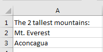
The formula values are now pasted as values in cell C1:

6. Delete columns A and B because we no longer need them.

Explanation of the Formula

The CONCATENATE function joins the several text strings in cells A1, A2, A3, and A4 into one text string.

The CHAR function returns the character specified by the code number from the character set of the computer. In this case, CHAR(10) returns a line feed/new line.

The REPT function repeats text a given number of times. In this case, REPT(” “, 5) repeats the space character five times.

Use CHAR function and code value 9

When we pass the value 9 to the CHAR function, it returns a Tab character in the Excel cell because the ASCII code for the Tab character is 9. The Tab character however will be invisible in Excel but it appears when we copy the data into notepad.

We will use the following dataset to explain this method:

We will use the following steps:

1. Select cell B1 and type in the formula:

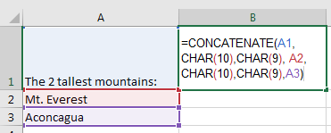
2. Press the Enter key:

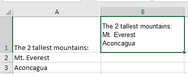
The Tab spaces are invisible in Excel but if we copy the data in cell B1 and paste it into Notepad the Tab spaces can be seen:

Use the Increase Indent button

We can use the Increase Indent button on the Excel Ribbon to give our data a “tabbed appearance.”

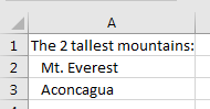
We will use the following dataset to demonstrate how we can achieve this:

We use the following steps:

1. Select cells A2 and A3.
2. Click Home >> Alignment >> Increase Indent:

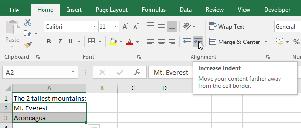
This Increase Indent command will push the content of our cells away from the cell border, giving our data a “tabbed appearance.”

Conclusion

It is easy to insert tab characters in word processors such as MS Word but in Excel, we cannot insert Tabs in cells. Pressing the Tab key in a cell simply moves the cell selector to the next cell on the right.

Tab spaces improve the readability and visual appeal of data and we may want our data in Excel to have the appearance of tabbed information.

In this tutorial we looked at four workarounds we can use to give our data in Excel a “tabbed appearance.”

We first looked at how we can manually add five spaces at the beginning of our data. This gives our data the appearance of tabbed information because one tab space is equivalent to 5 regular spaces.

We can also use the combination of CONCATENATE, CHAR, and REPT functions to add the five spaces to our data.

We also explored the use of the CHAR function and the code value of 9. This method adds invisible tab characters to cells.

Lastly, we looked at how we can use the Increase Indent button on the Excel Ribbon to push the data away from the cell border and achieve a tabbed appearance.