In so many examples that we’ve shown, we’ve proven how useful highlighting cells with conditional formatting can be.
In the text below, we will show how to use conditional formatting to highlight percentages in our data.
Highlight Percentages with Conditional Formatting
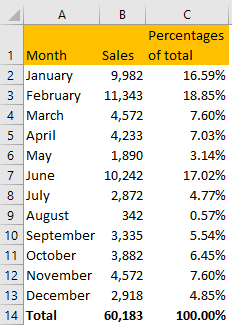
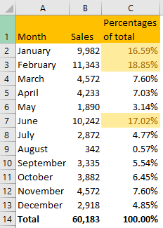
For our example, we will use a table with sales figures for every month and percentages of each sales figure in total.
Formula to get percentages of the total in the table above:
|
1 |
=B2/$B$14 |
We locked cell B14 (cell with total) to drag our formula till the end of the data set.
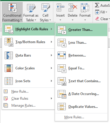
To highlight only the cells with percentages higher than 10 percent, we will select the range C2:C13 (excluding total) and go to Home >> Styles >> Conditional Formatting >> Highlight Cells Rules >> Greater Than:
On a pop-up window that appears, we will input 10 percent:
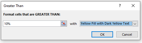
Once we click OK, our table will look like this:
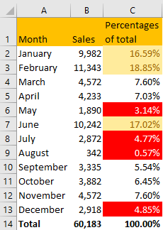
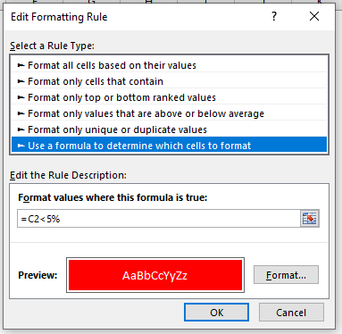
We can also highlight our cells with the formula of our choosing. Let’s say that we want to highlight the percentages lower than 5 percent with red color. To do this, we will select the same range and go to Home >> Styles >> Conditional Formatting >> Highlight Cells Rules >> More Rules.
On a pop-up window that appears, we will select the last option- Use a formula to determine which cells to format, and input the following formula:
|
1 |
=C2<5% |
Our window will look like this:
When we click OK, we will see that these changes are applied in our table and that all the cells with percentages lower than 5 percent are highlighted: