Highlight Negative Numbers in Excel

In Excel, there are limitless ways to highlight and mark only certain data in the data set. There are different ways to do so, as well.

In the following example, we will show different ways to highlight only negative numbers in the range.

Highlight using Conditional Formatting

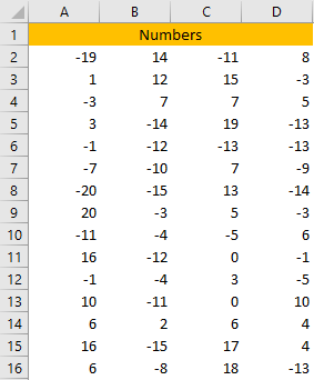
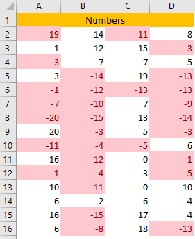
For our example, we will use a simple numbers table with four columns and random numbers from -20 to 20.

To create this table, we used a very useful formula called RANDBETWEEN. It has only two parameters: bottom and top. For our bottom number, we choose -20, and for our top number, we chose 20. So, our formula looks like this:

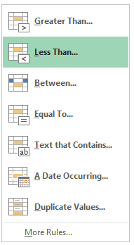
Now, all we have to do to highlight only the negative numbers in our data set is select our range, then go to Home >> Conditional Formatting >> Highlight Cells Rules >> Less Than:

In the pop-up window that appears, we will input the number 0, since we want to highlight all the numbers that are lower than this one.

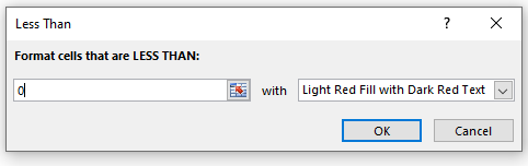
We will choose a standard fill – Light Red Fill with Dark Red Text, and then click OK.

Our table now looks like this:

Highlight using Filter

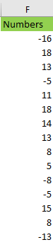
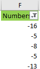
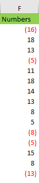
We will add this list of random numbers to column F as well. It would look something like this:

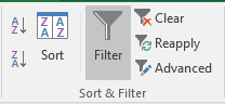
If we want to filter only the negative numbers from the list, we can do that by selecting the first row in our column, and then going to Data >> Sort & Filter >> Filter.

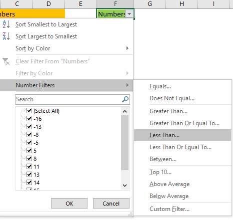
Once we click on the Filter, we will select the dropdown arrow in our column, go to Number Filters, and then select Less Than.

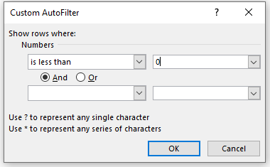
In the Custom AutoFilter pop-up window that appears, we will input 0 next to the “is less than” text.

We will click OK, and we will see that only the negative numbers are filtered out:

Highlight using Formula

We can also use a formula to derive the negative numbers in our data set. We will clear the filter in column F by going to Data >> Sort & Filter >> Clear.

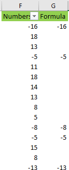
We will create a simple formula in cell E2:

This formula will copy negative numbers from column F and leave a blank space if the values in column F are higher than 0. We will copy the formula till the end of our data set in column F. Results are as follows:

Highlight using Formatting

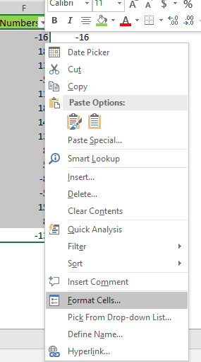
We can also use formatting to help us highlight negative numbers. We select our range (numbers in column F), right-click on it, and then select Format Cells:

In the pop-up window that appears, we have to make several adjustments.

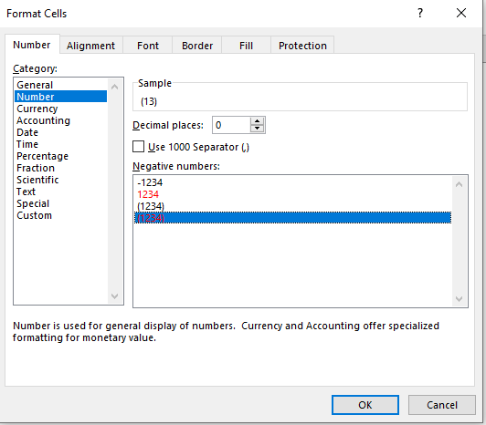
First, we select a Number as a category. Second, we set decimal places to 0, to avoid them (we defined our numbers as whole numbers, so there is no need for decimals). Next, we come to the best part. We can choose how we want to highlight our negative numbers.

In this case, we decided to highlight them with red color and to put them into parentheses (fourth option on the list).

When we click on OK, our range will look like this:

The same result could be achieved by defining this in the Custom category in Formatting.

To prove that, we will select our range once again, go to Format Cells, and then select the Custom category.

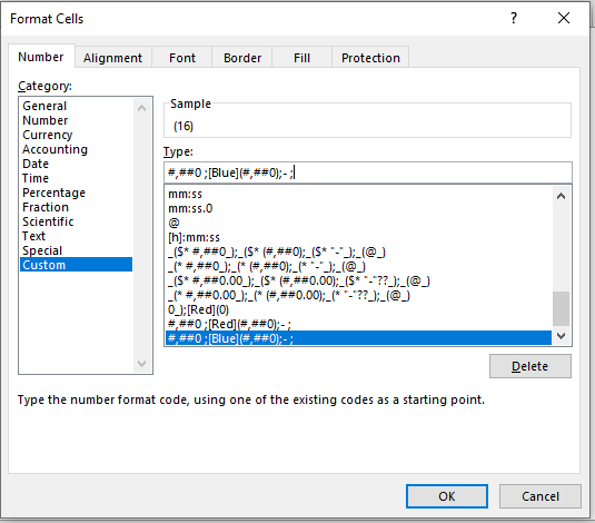
We will input the following syntax:

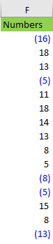
Now, our negative numbers should be highlighted in blue and should be in parentheses.

When we click OK, we will see that this is the case: