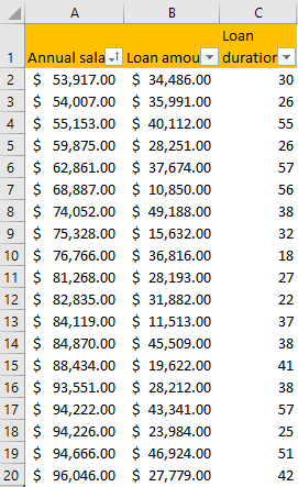
Suppose that we have an Excel table that has three columns: annual salary, loan amount, and loan duration.
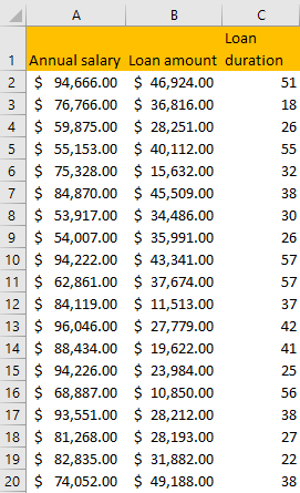
This table does not have many rows, and if somebody would like us to tell them the smallest number in each column, we could probably just go and find these cells with a “naked eye”.
However, that alone seems like a lot of work. Now imagine that our table was even larger. Luckily, there are a couple of ways to find the values we need. In this case, the smallest and the highest number.
Smallest and Largest Number with Filter
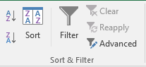
The first option is that we select the first three columns in our first row (the one that contains the names of our columns) go to the Data tab, then to Sort & Filter subtab, and then click Filter:
We will notice that our cells in the first row now have a dropdown list.
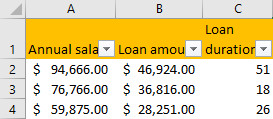
If we select the dropdown button in cell A1, we will notice a couple of options at our disposal:
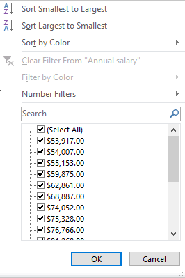
We can immediately figure out that we have our two desired options:
- Sort Smallest to Largest
- Sort Largest to Smallest
If we click on the first option, we will notice that our first column is now ordered from the smallest annual salary to the largest one.
Logically, as we have only chosen a dropdown from column A this is the column from which these values were ordered.
Now we know our highest and lowest value. We can do the same thing for other columns as well.
Smallest and Largest Number with Conditional Formatting
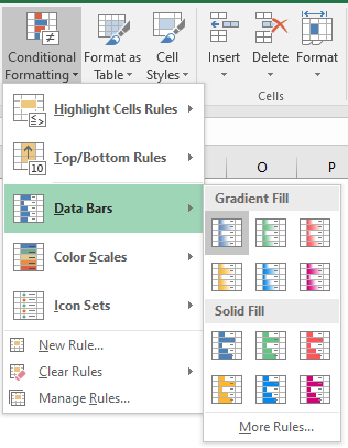
One more way in which we could find the largest and smallest value is the Data Bars option in Conditional Formatting.
We will select column B and then go to Conditional Formatting >> Data Bars and then choose the first option in Gradient Fill.
Cells in column B will now be filled automatically with the smallest value being the least populated one with blue color, while the largest value will be completely colorized.
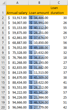
This option is pretty convenient when we operate with a smaller set of data, or we want to show our data using better graphics, but it is pretty hard to find the smallest and the largest values in this way when dealing with a large set of data.
Smallest and Largest Number with the Functions
The easiest way to find the smallest and largest values in our range is to use functions. Let us suppose that we want to find the smallest value in our column C (Loan duration).
We will go to the one cell below our final populated cell in the column (in our case cell C21).
There is also easier to go to the last cell in our range. We just click CTRL + Down Arrow and Excel will direct us to the last cell in our range.
After we found our cell, we will go to the Home tab, to the Editing subtab, click the arrow next to AutoSum, click Min (calculates the smallest value) or Max (calculates the largest value), and then press ENTER.
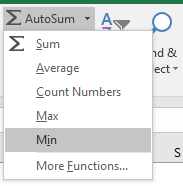
If we click on Min, we will automatically be presented with a function that Excel prepared for us:
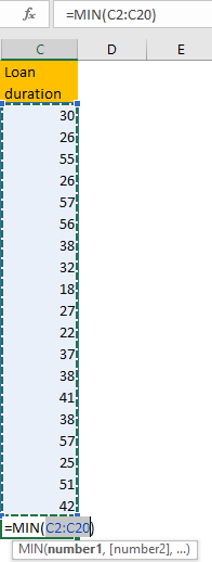
As we can see, our function seems fine. We will click ENTER and then we will be presented with the result, which is, in this case, the number 18.
To find the highest value, we have to change our function from MIN to MAX.
Smallest and Largest Number with VBA
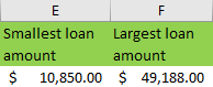
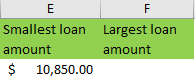
Since we did not resolve the issue of the smallest and largest value in column B, we will do it with the VBA code. For this, we will define cell E1 as the Smallest loan amount and cell F1 as the Largest loan amount .
We will input the smallest value of the column B in cell E2 and the largest value of column B in cell F2.
Our VBA code will be as following:
|
1 2 3 4 5 |
Sub Return_lowest_number() Dim ws As Worksheet Set ws = Worksheets("Loan table") ws.Range("E2") = Application.WorksheetFunction.Min(ws.Range("B2:B20")) End Sub |
In the first part of the code, we declare the variable. Dim is short for dimension and we use it when we want to declare a variable, which will be remembered and can be used later in our code.
For our example, we are creating the variable ws which will be defined as a worksheet.
In the next step, we are setting our variable to refer to our worksheet. Our worksheet name is Loan table, so we will set our variable ws to be equal to this name.
Finally, we call out our variable, and then we put a dot (“.”) that will allow us to call a specific cell from our worksheet. In this step, we define the cell in which we want to input the data and then we define the data itself. Our desired cell is cell E2.
We want our E2 cell to be equal to the minimum value of range in the column B. On the other side of the equation, we first call for our application, so that we can call for the worksheet function as well. Next, we call for the Min function, to return the minimum value of our range.
Then, we want to define our range. Our range will obviously be located in our sheet, and we call our variable for the sheet and then we call for the range of our data, which is B2:B20.
When we run our code with F5, we will get the result in cell E2 as follows:
To return the highest value, i.e. largest loan amount, we have to make some adjustments in our code. We will create another code beneath our first one and it will look like this:
|
1 2 3 4 5 |
Sub Return_largest_number() Dim ws As Worksheet Set ws = Worksheets("Loan table") ws.Range("F2") = Application.WorksheetFunction.Max(ws.Range("B2:B20")) End Sub |
As seen, we changed the name of our code so is now Return_largest_number.
Next, we have changed our output range, by changing the cell reference (“F2”), in our code.
Our range remained the same (B2:B20), although we could change this if we wanted as well.
Finally, we changed our function from Min to Max.
Our table looks like this: