Although it is very hard to capture everything about the Pivot Tables in Excel, we tried to do that in previous topics. One thing that was not discussed was filtering the multiple values in these tables.
We will cover this one in the text below.
Filter with Pivot Table Fields
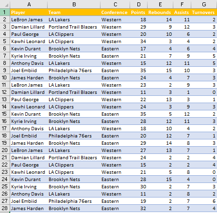
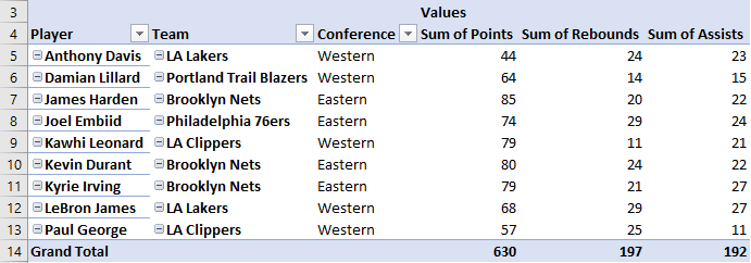
For our example, we will use our well-known table of NBA players and their statistical categories (points, rebounds, assists, and turnovers) from three nights:
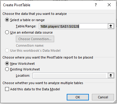
We will now create our Pivot Table by selecting the range A1:G28 and going to Insert >> Tables >> Pivot Table.
On a pop-up that appears, we will simply click OK and our Pivot Table will be created in the new sheet:
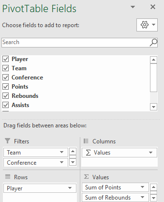
We will insert our players into the Rows fields, and the sum of points, the sum of rebounds, and the sum of assists into values. Pivot Table already has a built-in function for filtering, so we will add team and conference into the filter.
The setup of our Pivot Table will look like this:
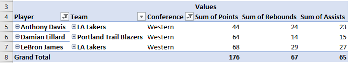
And our Pivot Table itself will look like this:
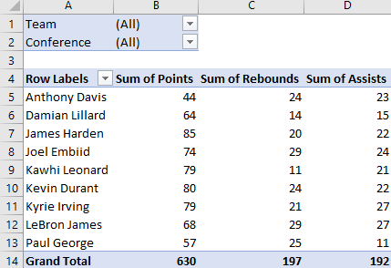
We can now choose the team or teams that we want, and a conference that we want. Now, logically, since we have only two options for conferences, when we choose the Western conference, it will limit our options:
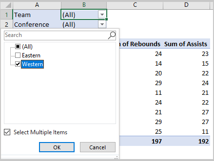
We clicked on a small dropdown at the right side of the word „All“, selected Multiple Items, then chose only Western Conference.
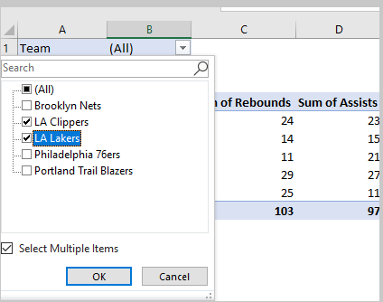
Now we will do the same thing for Teams. We will notice that, sadly, we are not left with only the teams from the Western Conference, but we rather have all teams available. We will select LA Clippers and LA Lakers since we know that these teams will return some results:
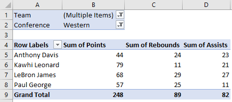
Our Pivot Table now looks like this:
Filter with Pivot Table Label Filters
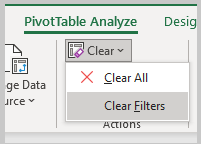
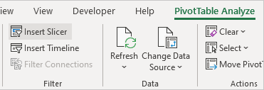
Now we will clear all of our filters. To clear them all out at the same time, we will click anywhere on our Pivot Table, then go to PivotTable Analyze field >> Actions >> Clear Filters:
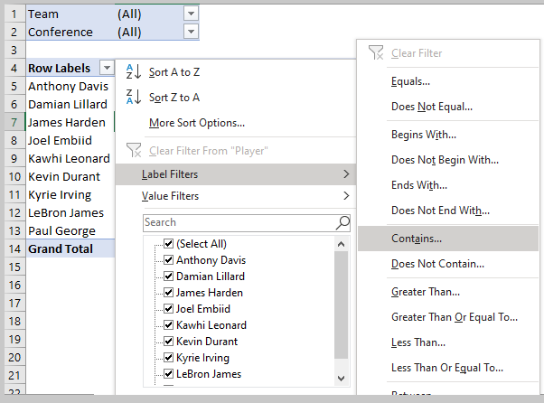
Once we do that, we will go to our Pivot Table, go to a dropdown at the Row Labels >> Label Filters >> Contains:
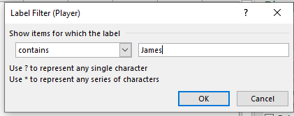
On a pop-up window that appears, we will input the word “James”:
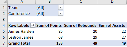
Our Pivot Table now looks like this:
Now, if we wanted to filter our only LeBron James, we can do it with the help of Value Filters.
Before that step, we need to include one important thing. We have to right-click anywhere on the Pivot Table, and select Pivot Table Options:
We will go to the Totals & Filters tab, and then select Allow multiple values per field:
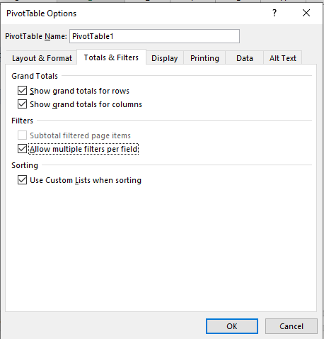
If we have not done this, then every other filter that we would create would simply replace our already created one. This way, the new filter will be added to the existing one.
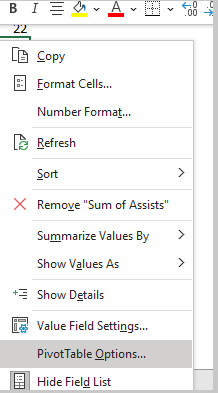
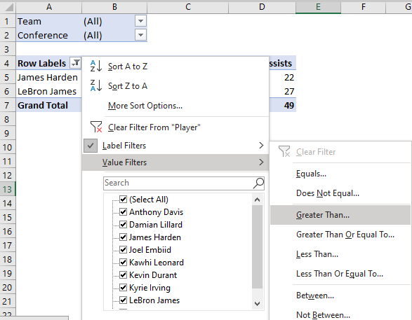
Now, we will select the dropdown arrow again, then go to Value Filters >> Greater Than:
On a pop-up that appears, we can choose between our three categories: points, rebounds, and assists. We will choose assists and input 25 (as James Harden has 22 in total, and Lebron James has 27).
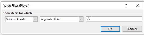
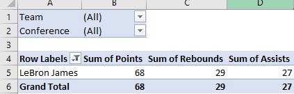
When we click OK, we will have only LeBron James selected in our Pivot Table:
Filter with Slicers
Another way to filter multiple values in Pivot Table is to use Slicers. We will create another Pivot Table with the same data. Then we will place player, team, and conference in rows fields and the sum of points, rebounds, assists in the values field.
To insert a Slicer, all you need to do is click anywhere on the Pivot Table, go to Pivot Table Analyze >> Filters >> Insert Slicer:
When we click on it, we will select the field that we want to be included:

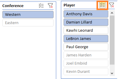
We will choose Conference, then repeat all the steps and select Player. When we get our Slicers, we will select a Western conference, and click on the Multi-Select button (marked with a red square in a picture below) to select a few players from this conference.
The great thing is that all the players that are not part of the Western conference are greyed out:
Finally, our Pivot Table looks like this: