Drop Down List in Excel

Drop-down lists are useful when it comes to selecting one item from multiple choices. They are very popular in online forms, especially for languages, countries, cities, etc.

But the web is not the only place you can find them; They can also be present on desktop applications.

Excel is one of them. It offers a pretty extensive set of tools that allows manipulating drop-downs in many different ways.

Prepare drop-down list of data

To use drop-down lists, you have to prepare data. It’s a good idea to place data in a different worksheet than drop-down lists. This will help you to organize it better and avoid accidental deletions.

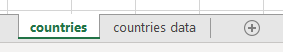
Inside our example, there are two sheets: “countries” and “countries data”.

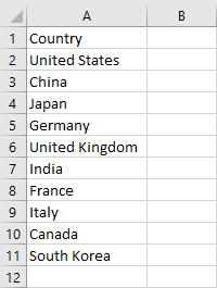
On the first tab, we are going to create a drop-down list, and on the second one, there will be a list of countries we are going to use.

Remember to remove blank spaces inside the source you are going to use for a drop-down list, otherwise, these blank spaces are going to appear inside the drop-down list.

Create a drop-down list

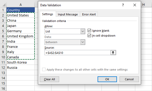
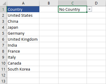
Click cell B3 and navigate to Data >> Data Tools >> Data Validation.

From the Settings tab, under Validation Criteria, select List.

After you do this, the source textbox will appear.

Click the arrow next to it, and select cells from cell A2 to A11. Be careful, not to choose the header, otherwise, it will be present inside the dropdown.

After you confirm your selection, it will appear in the source box.

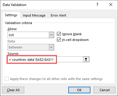
Click OK to insert the drop-down.

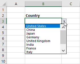
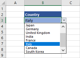
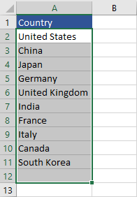
At first, it seems that nothing happened, but if you click the cell, you will notice that there is a small button with a triangle inside. Click it to show all the options.

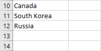
The problem with this approach is that it’s not dynamic. If you add another country at the end of the list, (A12) it won’t appear inside the drop-down.

To fix this problem you can do one of two things: You can change the formula inside a validation window or you can create a table from the data and then and then define a name for it.

But changing the formula each time is very tedious and it’s not the way we are supposed to work with Excel, so we are left with the second option.

Using tables with defined names

Click any cell on the second sheet with data, and navigate to Insert >> Tables >> Table or the Ctrl + T keyboard shortcut.

A new window called Create Table will appear.

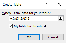
Make sure that you have My table has headers selected, otherwise, Excel will create a header for you, and the word “Country” will be inside the drop-down list as one of the countries.

Naming the table

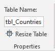
To name a table, first, you have to click it. A new special tab, called Table Design will appear. On this tab, under Properties, you can change the table name. I called it “tbl_Countries”.

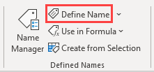
Define a name

After you defined a name for the table, Now, it’s time to define a name for table data.

Select all cells, except headers, inside a table (A2:A11) and navigate to Formulas >> Defined Names >> Define Name.

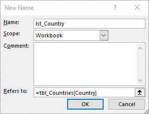
Name the new range “lst_Country”, and set a reference to “=tbl_Countries[Country]”. Because we want to use it on the first worksheet, leave Scope as is.

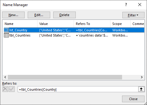
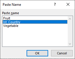
You can check and edit defined names in the Name Manager, under Formulas >> Defined Names.

And indeed, there is our table and range we’ve just defined.

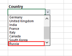
Let’s move back to the first sheet and add the new drop-down. It’s going to look like this:

When you have a mouse cursor inside the Source textbox, you can press F3 and choose one of the created lists.

To see how it works, add a new country at the end of the list.

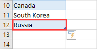
This new entry will be automatically added to the dropdown list.

Sorting

You can’t sort a drop-down list after you create it, but you can sort the table, and the drop-downs that use it as a source will be automatically updated.

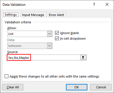
Entering data manually

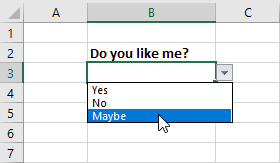
If you have a drop-down list with a few items that don’t change, instead of using a list of cells, you can add values inside the Source textbox.

Click OK to see that these three values are inside a cell as a dropdown list.

It’s good to know that you have this option, but since you already have a sheet with drop-down elements, it’s better to keep them there so you have all your data in the same place.

Input messages and error alerts

With a drop-down list, you can give users some guidance on what to do when they click it. These are input messages and error alters.

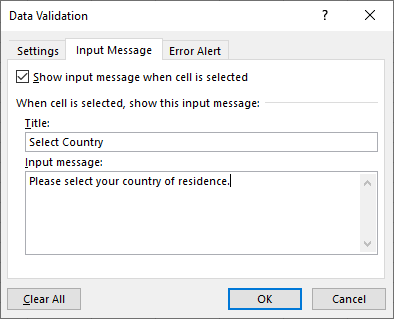
Input Message

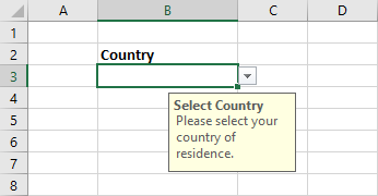
The input message is just a hint for a user – a simple message on what to do with a drop-down.

Click OK. Now, the message will appear when you click a cell with the drop-down list.

If you have a lot of similar drop-down lists, it may be wise to add just one or two, as repeating the same message many times can be irritating to a user.

You can press Esc or click away from the cell for a message to disappear.

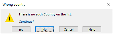
Error Alert

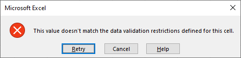
Instead of choosing from the drop-down list, you can type a name, but if you enter a value that is not on the selected list, you will receive a generic error message.

To override this message, you can write the specific one for the list.

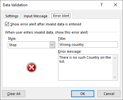
This error alert works the same as the previous one, but with a different message.

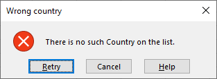
This entry will not be accepted, so you have to click Cancel and type and reselect something that is on the list.

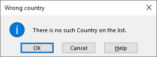
Warning and Information

The warning and information messages are very similar. Contrary to the Stop alert, which doesn’t allow you to enter data. These messages will only display information that the value you’ve just entered is not present on the list. You have the option to enter the value anyway.

Warning

The warning is information that the creator of this drop-down probably thinks you made a mistake while typing, but you can add it anyway if you are sure of your entry.

Information

This is just a hint. It’s less strict than a warning message.

These messages are optional but may be helpful in some cases when you may feel that it will help users.

Add/remove items

A drop-down list is usually connected to a table. If you want to do operations such as adding and removing items, you have to do it there.

To add an element to a drop-down list, add one at the end of the table.

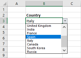
To add an entry in a particular position, you have to use an insert feature. Let’s say you want to add Spain between France and Italy, right-click the row number (9) and choose Insert.

There is an empty position between these two rows. You can add “Spain” there. It will be reflected in the drop-down.

Remove a drop-down list

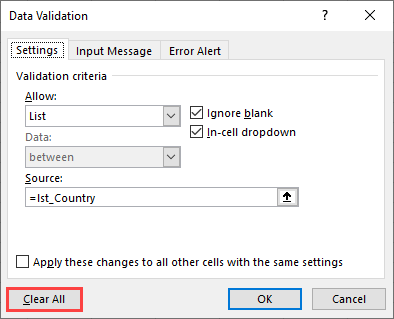
You can remove single or multiple drop-down lists at once. Select cell or cells with dropdowns and navigate to Data >> Data Tools >> Data Validation. In the bottom-left corner, there is the Clear All button.

Format

Formatting drop-down lists look the same as formatting any other cells. It will be applied only for the selected cell and not for those inside a drop-down list.

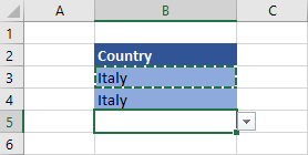
Copy

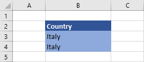
There are two ways to copy drop-down lists. The first one is to use Ctrl + C and then Ctrl + V. It will copy a list and visual formatting.

If you want to copy the drop-down list without formatting, copy the cell and instead of standard pasting, use Paste Special.

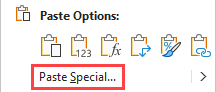
From the Paste Special options, choose Validation.

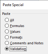
The value is pasted without formatting.

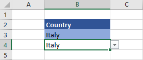
You can also copy the drop-down list with formatting and then use Format Painter (Home >> Clipboard). After you click Format Painter, click an empty cell and then drop-down. It will format the drop-down in the same way as an empty cell – without formatting.

Apply changes to all other cells

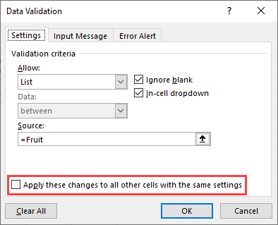
After you copied the same drop-down list into many cells, you want to change it. You can either do it for a single or multiple drop-downs you’ve copied.

Choose one drop-down and click the Data Validation button. At the bottom of the window, there is an option. Uncheck it if you want to change a single drop-down, or check it if you want to make changes to all copied drop-downs.

Security

We usually place data used in a drop-down list on the second sheet. You may want to protect this worksheet, so nobody can make changes to it.

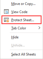
To do it, select a sheet you want to restrict, and navigate to Review >> Protect >> Protect Sheet.

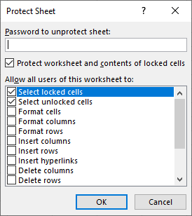
You can add a password, otherwise, people can unprotect it.

You can also right-click the worksheet tab and select Protect Sheet.

Fix potential problems

There are a few problems you can face when you work with drop-down lists.

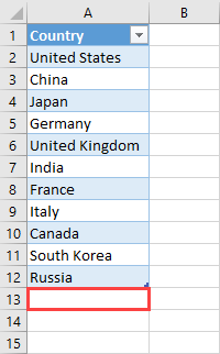
Missing Items in Drop Down

If you define a range for table elements as you did before, you shouldn’t encounter any problems. You can encounter them if you add an element to the normal range, and you forget to change source data.

As you can see, the source had been selected before the last two options were added that’s why they are not present inside a drop-down list.

Apart from changing the source each time or using tables, there is a third option to deal with this problem.

The last option is to select the whole column.

But you can’t type just =A:A when you have a header because it will be added to a drop-down list. Instead, use the formula with the OFFSET function.

This formula adds all cells from column A, but the first one (header).

Now, when you add additional elements they will be visible inside the drop-down.

Entering any value

By default, you can’t enter values into a drop-down list that are not present inside the source. Even if you create a drop-down list with empty cells. But look what’s going to happen if you define a name for a list.

Now, if you add this selection as a source of a drop-down and try to type a value that is not present, you are going to get an error, but Excel behaves differently if you give this range a name and try to use it instead of a range.

Select cells from A2 to A12.

Navigate to Formulas >> Defined Names >> Define Name and call it “withEmptyCells”.

Create a drop-down using this name.

Now, if you try to enter any name it won’t return an error.

It will return an error if you enter as a source the same range or you name a range without any empty cells inside.

There is an option you can check which will force Excel to return an error. In the Data Validation window, you have to uncheck the Ignore blank checkbox.

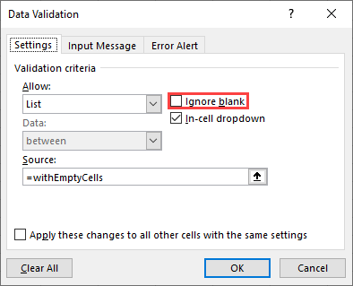
Now, if you try to enter a value that is not on the list, you will get an error.

Case sensitive

If you enter values that are not inside the drop-down list, you will get an error. But it doesn’t mean that you have to enter them using the same case.

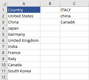
You can use whatever case you want, even some weird ones, and Excel is not going to complain.

But there is an exception.

If you type a list of options directly inside the source textbox. You have to enter the exact case in the drop-down.

Now, if you type one of these values, Excel won’t complain. But if you use a different case, you will get an error.

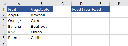
Dependent Drop-down Lists

Dependent drop-down lists are the lists where one drop-down is dependent on another.

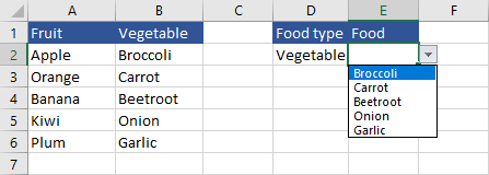
In the following example, we are going to select a food type: fruit or vegetable. Next, depending on this choice, the other drop-down will display the relevant data.

Let’s use the following example:

First, under the “Food type”, we are going to add a drop-down.

Click cell D2 and add a new drop-down list. In the Source choose =$A$1:$B$1.

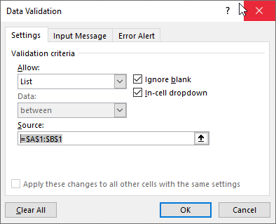
The first drop-down is active.

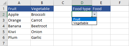
Now, it’s time to create the second one.

This time select the entire table (A1:B6). Go to Formulas >> Defined Names >> Create from Selection.

From the new window, we want to uncheck the Left column because we want named ranges for fruit and vegetable types, and not for each fruit.

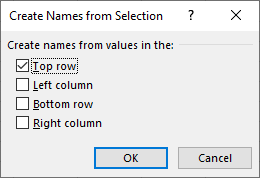
Now, if you go to the Name Manager, you are going to find two additional named ranges: Fruit and Vegetable.

Click cell E2, and open Data Validation. Enter the formula with the INDIRECT function.

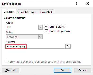
the INDIRECT function takes a text reference as an argument; For example, =INDIRECT(“B3”) returns “Carrot”. Depending on the drop-down value we choose, we have either Fruit or Vegetable, and the function returns these named ranges created before.

If you haven’t chosen an option from the “Food type” list, you are going to get this message:

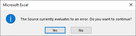
Click Yes, and the second drop-down will start working the moment you choose a value from the first one.

Vlookup to fill data

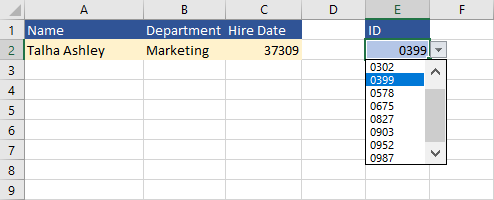
Sometimes, when a user selects a drop-down element, he doesn’t need to fill in other data. For example, if he chooses employee ID, which is a unique value, other fields should automatically be filled.

We are going to do it, using the VLOOKUP function.

This is the table we are going to use.

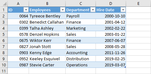
Let’s name it “tbl_Employees”.

Now, it’s time to create a drop-down from IDs and fill in other data.

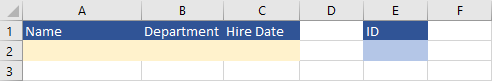
Under “ID”, in cell E2, insert a drop-down with IDs from the table (A2:A10).

Inside cell A2 enter this formula:

It’s going to check cell E2 from the current worksheet, which is “ID”, and return value from the second column in the same row of the table “tbl_Employees”.

For B2 and C2 insert these formulas:

The IFERROR function makes sure that if the formula returns an error, it will leave the cell empty.