Create Pivot Table in Pivot Table

Usually, we create Pivot Tables from tables, but you can also create a Pivot Table from the data inside another Pivot Table. In Excel 2003 there was a wizard to create Pivot Tables or Pivot Charts.

This wizard still exists inside Excel, but it’s hidden. In this lesson, I’ll show you, how you can use it, and also how you can add it to your Quick Access Toolbar, so you are going to have quick access to it any time you want.

Create a Pivot Table inside another Pivot Table

I’m going to use the following table.

1. Create a pivot table from the table.
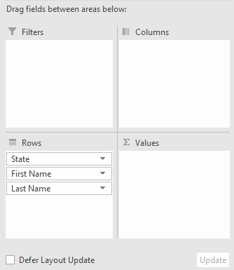
2. Select all Pivot Table fields and move them to Rows, so the State is at the top.

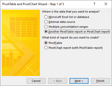
3. Press Left Alt (don’t hold), then d, and then p to open Pivot Table wizard.
4. Select Another PivotTable report or PivotChart report.

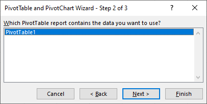
5. Choose the Pivot Table, you want to use.

6. Choose the cell where you want to place the new Pivot Table.

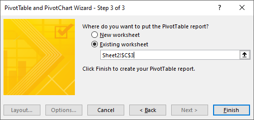
7. Place Finish to create the new Pivot Table.

After you place it, you can click the Pivot Table fields as you did in the previous Pivot Table.

Adding Pivot Table wizard to Quick Access Toolbar

If you don’t want to memorize these keyboard shortcuts, you can easily add this wizard to Quick Access Toolbar.

1. Click the icon.

2. Click More Commands.
3. Choose Commands not in the Ribbon.
4. Search for PivotTable and PivotChart Wizard.
5. Click OK.

A new icon appears in Quick Access Toolbar. Now, you can quickly use it without the need of memorizing keyboard shortcuts.