We already showed how useful Pivot Tables can be, how to filter our data in these tables, how to arrange our data, and how to use Slicers with them.
However, we did not discuss how we can implement a formula in the Pivot Table. In the example below, we will show exactly this.
Create a Formula in Pivot Table
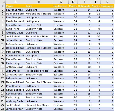
To show the formulas, we first need to create a Pivot Table. We will make it out of our table with NBA players and their statistics from several nights- points, rebounds, assists, and turnovers.
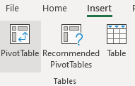
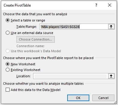
To create a Pivot Table, we will select the range A1:G28 and go to Insert >> Tables >> Pivot Table:
On a pop-up window that appears, we will click OK, and our table will be created in the new sheet.
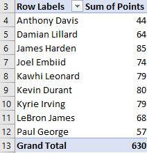
We will call this sheet simply “Pivot Table”. Then we will put the Players in Rows fields, and Points in value fields:
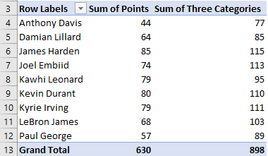
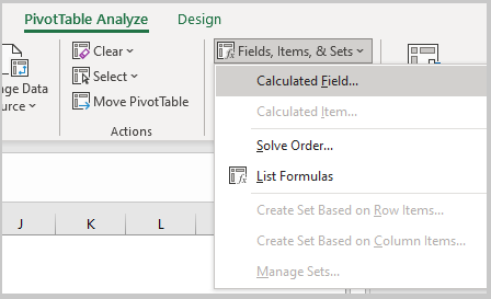
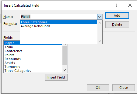
Let us now suppose that we want to know the sum of three categories: points, rebounds, and assists. To do so, we will click on our Pivot Table, then go to the PivotTable Analyze tab >> Calculations >> Fields, Items, & Sets >> Calculated Field:
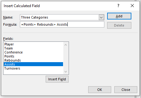
When we click on it, we will be presented with a pop-up window on which we will choose the name of our new field (we named it Three Categories) and we will define our formula (in our case points + rebounds + assists):
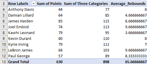
We will click OK, and our new field will be added to our Pivot Table:
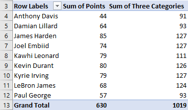
We can see that our three categories have been summed.
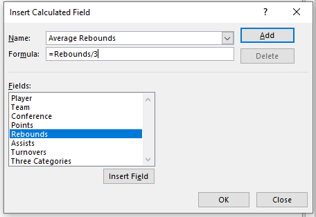
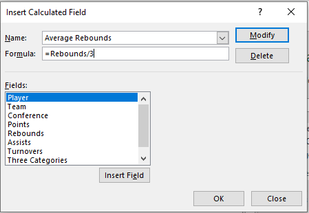
We can do various other calculations. Since we know that our original table covers three game nights, we will calculate the average number of rebounds per player.
To do so, the same steps will be taken. Our formula will look like this:
We will click Add, and will have the following results in the Pivot Table:
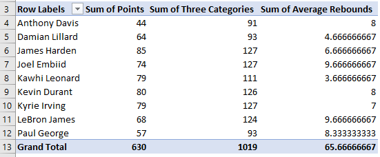
We can see that we have a Sum of Average Rebounds field because the custom formula when adding any field to the Values is “sum”.
This is, so to say, a mistake in naming convention since the values shown in this column are averages of rebounds for every player.
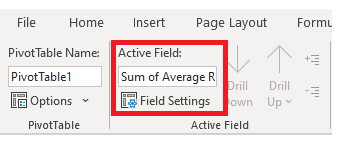
We can change this by clicking anywhere on the field, then by going to the PivotTable Analyze tab >> Active Field and changing the name:
View, Edit, and Delete a Formula in Pivot Table
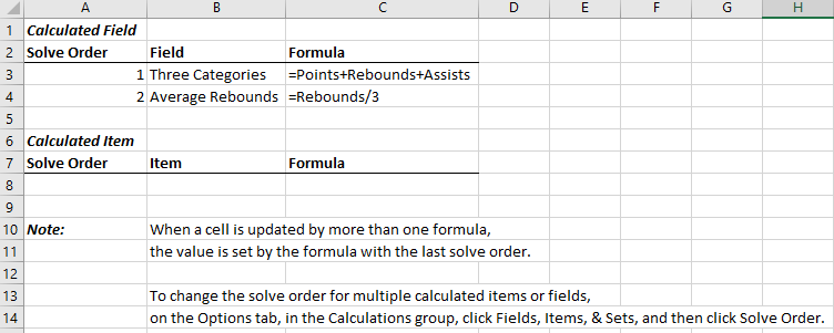
To view all the formulas that we created, we will again go to the PivotTable Analyze tab after clicking anywhere on the table, then to Calculations >> Fields, Items, & Sets >> List Formulas:
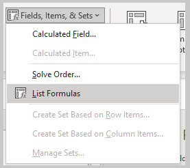
When we click on it, we will have the list of our formulas in another sheet:
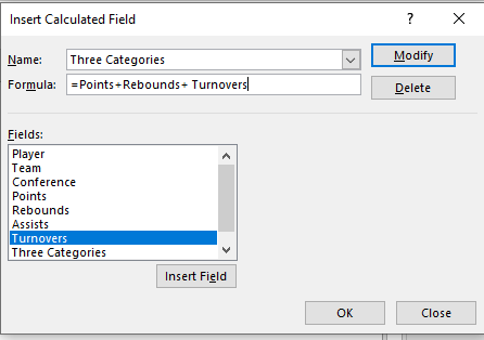
If we want to change our formula for whatever reason, we will click on the table and go to the PivotTable Analyze tab >> Calculations >> Fields, Items, & Sets >> Calculated Field (same steps as we entered the formula for the first time).
Under the Name field, we will find our formula (Three Categories in our case):
We will click on it, we will change assists with turnovers, and click on the Modify button:
Now our table has a different set of values:
In the same way that we edited our formula, we can also delete it. We will repeat all of our steps but for the final one (we will select the Average Rebounds formula now). Instead of clicking on Modify button, we will click Delete:
We now have our Pivot Table altered, i.e. one column was deleted: