Convert Rows to Columns in Excel

Rearranging data from rows to columns or columns to rows is called transposing. It’s useful when you want to change the structure of a worksheet.

Instead of doing it manually, Excel offers a feature called “Transpose” that will take care of the task.

In this example (ConvertRowsToColumnsInExcel.xlsx), the data I showing how many hours our employees worked in the first six months of the year.

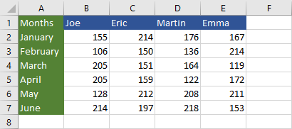
Later we decided, that we want months to be placed horizontally and names vertically.

To do it, select all the cells inside the entire range (A1:E7) and copy them (Ctrl + C).

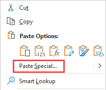
Right-click cell A10 and click the transpose icon.

Now, the months are inside a single row and names inside a single column.

Transposing is not available for tablets. If you have a table, first, you will have to convert it to the range. To do it, click a table and navigate to Table Design >> Tools >> Convert to Range.

Transposing with different formatting options

The cells you transposed so far copied everything from the source data: fonts, formatting, width, etc.

The Paste Special… feature gives you a bit more flexibility.

If you copy the range, then, instead of clicking the transpose icon, click Paste Special….

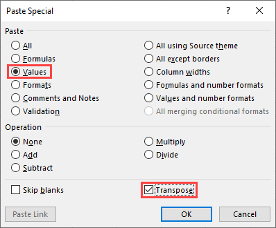
Now, you can select whether you want to paste everything, or maybe just formatting. In this case, we are going to paste only values, without formatting.

Don’t forget to select the Transpose checkbox.

Now, you have the same data, but without formatting.

TRANSPOSE Function

There is also a function called TRANSPOSE that converts a vertical range of cells to a horizontal and can be used instead of copying and pasting.

Enter the following formula inside cell A10:

It will transpose the data without formatting.

To remove the entire range, you have to delete cell A10.

The advantage of this function over the standard copy and transpose is that it’s dynamic. If you change one value inside the source data it will automatically change in the transpose function.

It’s very useful, especially when you want to transpose it between different sheets.

Shortcut for transposing

You can quickly copy transposed data by creating a macro and applying a shortcut.

Here’s how you can do it.

First, copy the data you want to transpose, then select a place where you want to insert the transposed data.

Now, it’s time to create a macro.

navigate to View >> Macros >> Record Macro.

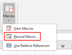
Inside the new window enter the name for your macro. Click the white square under the Shortcut key and press Shift + T. This will assign Ctrl + Shift + T to your macro. Click OK to start recording.

Right-click a cell and choose the transpose icon.

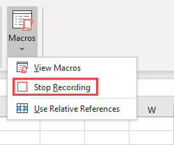
Navigate to View >> Macros >> Stop Recording.

If you want to see how your macro looks like, go to View >> Macros >> View Macros.

And there it is, the myTranspose macro.

Click Edit to see how it looks like, or click Cancel to close the window.

This is how the code looks like:

There are a macro name and comment with information about the shortcut assigned to this macro.

At the end of the function, there is a line that copies everything, and transpose is set to true.

Let’s check how our macro works.

Copy cells you want to transpose, and click a cell where you want to place the new transposed cells.

Now, you can use the keyboard shortcut we created earlier (Ctrl + Shift + T).

Now, you can transpose data with a quick keyboard shortcut.

You can modify the code if you want to transpose data without formatting. If you don’t know how to do it, you can create another macro paste special and look at the VBA code that is generated by Excel.