We already explained how exactly are Pivot Table and Pivot Chart slicers created. We also discussed that slicers are interactive filters of our data set.
In the following example, we are going to show how these slicers can be connected with multiple Pivot Tables, with the presumption that two or more of them have been created.
Connect Slicers to Multiple Pivot Tables
As in the previous example with slicers, we will use the list of NBA players, their teams, conferences, and statistics from several matches.
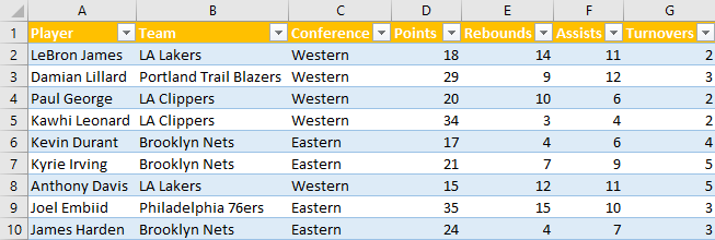
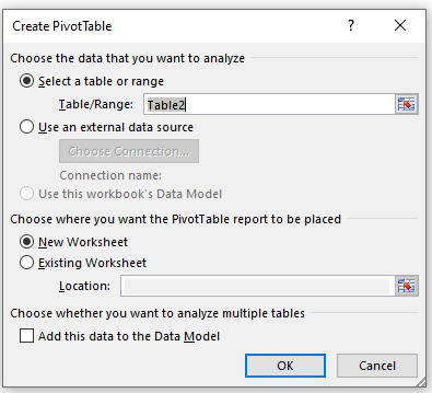
Next, we will create two Pivot Tables, by selecting our data set (the data set has 28 rows, but only 10 are presented in the table below), and going to Insert >> Table >> Pivot Table.
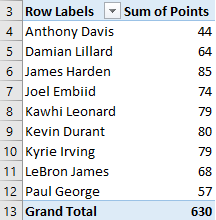
In the first Pivot Table, we will select only the list of players and the sum of their points. It will look like this:
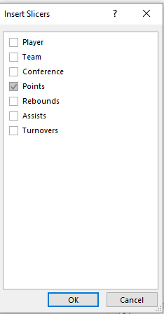
Next, we will create a Slicer by selecting any data in the Pivot Table, then going to Pivot Table Tools >> Analyze >> Insert Slicer.
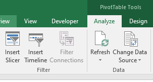
When we select the icon, we will only select the points as our Slicer.
Next, we will create another Pivot Table with the same data set and in the same sheet.
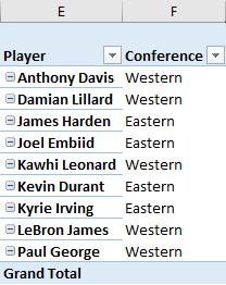
For this table, we will only have Players and Conference in rows fields.
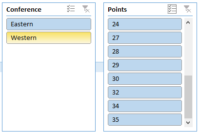
We will insert Slicer and choose Conference this time.
Now we have two slicers:
To connect them, we have to right-click anywhere on the first Slicer and select Report Connections.
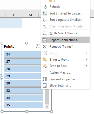
When we click on it, a pop-up will appear with the option to select and connect our Pivot Table with different existing Pivot Tables.
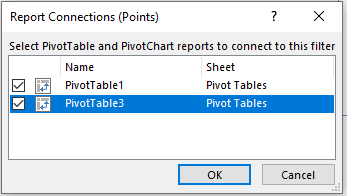
In our case, we can only connect our PivotTable1 with PivotTable3. We click on it and now are two tables are connected.
Next, we have to click on the second Slicer and do the same thing:
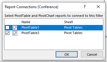
When we select the connection for the second Slicer as well, we can say that they are fully connected.
To see what exactly we have achieved, we will only select the Eastern conference in the second Slicer, and have the following data in our tables:
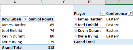
You will notice that, by selecting only the Eastern conference in one Slicer and the second Pivot Table being filtered, our first table will change and only the players from the Eastern conference will be shown. This has been changed even though we did not choose conferences in fields in the first table.