Conditional Formatting in Excel

We already explained where the Conditional Formatting is located in Excel, and that it can be used to highlight cells or a range of cells based on certain criteria.

In the following example, we will see how it is used with various criteria.

Conditional Formatting Based on Text

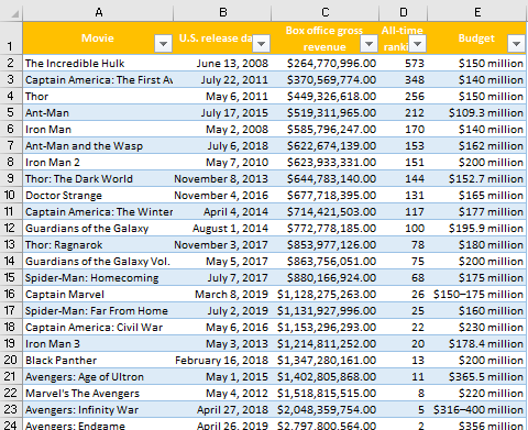
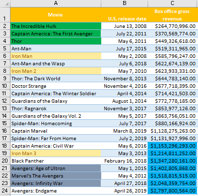
For this example, we will use the table of Marvel movies, with their release date, box office gross revenue, all-time ranking in revenue, and budget.

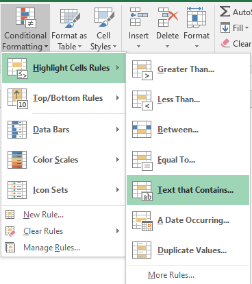
Now let us say that we want to highlight only the cells in the A column that contains Iron Man. We will select A column, go to the Home tab >> Conditional Formatting >> Highlight Cells Rules >> Text that Contains. 

After we click on this option, a pop-up will appear, on which we will input our desired criteria- Iron Man beneath Format cells that contain the text option:

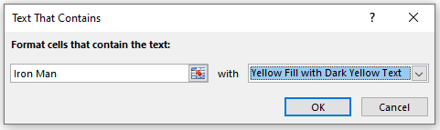
We will highlight all the cells that contain our criteria with yellow fill with dark yellow text.

Iron Man movies now look like this in our table:

Conditional Formatting Using Formula

We can also use a formula to define the criteria that we want to be highlighted. For the use of this example, we will input our desired criteria in cell G2. This will be the text: Avengers. 

We select A column again, Home tab >> Conditional Formatting >> New Rule.

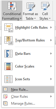
On a pop-up window that appears, we have to select the last option: Use a formula to determine which cells to format:

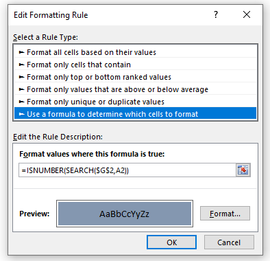
Then, we have to define our formula, in this case:

This formula searches for our criteria value in cell A2, which is the first cell in our table where we want to check if our criteria are met. 

Since our desired criteria are always the same, cell G2 has to be locked using the F4 button on a keyboard. 

Once we define our formula, we click on Format where we can customize the look of the cells that contain our criteria.

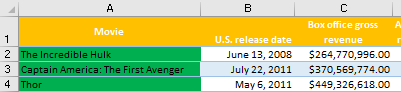
We click the OK button, and we have our Avengers movies highlighted.

Conditional Formatting Based on Text or Value in Another Cell

We can also base our criteria on some text or value in another cell. For example, we know that we have box office revenue for our list of movies. We want to highlight all the movies names (in column A) whose revenue was lower than $500 million (column C).

Since we already ordered our movies from the lowest revenue ones to the highest, we already know that the first three movies on our list will be highlighted.

We use the same step as in the example below, i.e. we select our range (A2:A24) and then go to Conditional Formatting >> New Rule >> Use a formula to determine which cell to format. 

Our formula will be:

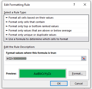
And we will format all of the cells in column A that meet our criteria with green color.

You will notice that the starting row in our formula is the same as the row of the first movie in the list (row number 2).

The first three movies in our table will be highlighted, as their revenue meets our criteria.

Conditional Formatting to Find Highest Values

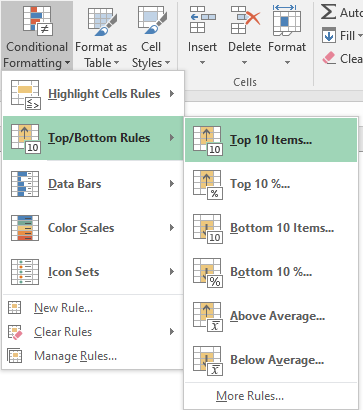
There are also options with Conditional Formatting that can automatically help us to determine or highlight the highest or lowest values in our data. We can choose how many of the lowest or highest values we want to mark. 

Let’s say that we want to find the top seven Marvel movies in terms of gross revenue. We will select our revenue column (range C2:C24). Once we do this we will go to Conditional Formatting >> Top/Bottom Rules >> Top 10 Items.

Once we click on it, we will be presented with a pop-up window, asking us to choose how many of the highest values we want to highlight (Format cells that rank in the TOP):

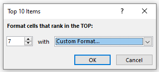
We will select seven, and then custom format our cells to be light blue. Since we have already ordered our movies by budget, our table’s final seven movies should be highlighted, which is true in this case.

Clear Rules

Conditional Formatting in Excel is a powerful tool, but sometimes, a sheet can become overloaded with formatting rules, making it difficult to interpret the data. This is where clearing rules comes into play.

There are two main ways to clear conditional formatting:

Specific Cells:

Highlight the desired cells, then navigate to Home >> Conditional Formatting >> Clear Rules >> Clear Rules from Selected Cells.

Press Alt + H + L + F to quickly clear formatting from selected cells.

Keyboard Shortcut

Entire Worksheet:

In a similar way you can clear rules from entire worksheet:

Go to Home >> Conditional Formatting >> Clear Rules >> Clear Rules from Entire Sheet.

Excel 365 Update

• New Data Bar Fill Options: Excel 365 offers a new option for Data Bars within Conditional Formatting. You can now use a gradient fill to represent data values. This provides a more visually appealing way to represent data variations.
• Icon Set Expansion: Excel 365 features additional icon sets for conditional formatting rules. These include icons designed specifically for temperature, weather, and progress tracking, allowing for more diverse visual representations of data.
• Formula Bar Enhancements: The formula bar experience for conditional formatting rules is improved in Excel 365. It offers:
  • Better suggestions: As you type your formula, Excel 365 provides more comprehensive and relevant function and reference suggestions.
  • Error checking: Excel 365 highlights any errors within the formula used in the conditional formatting rule, aiding in creating accurate rules.