Pivot Tables are one of the most useful tools that are available in Excel. We already showed how to create them, edit them, and delete them.
In the example below, we will show how to add and remove Pivot Table Formatting.
Add Pivot Table Formatting
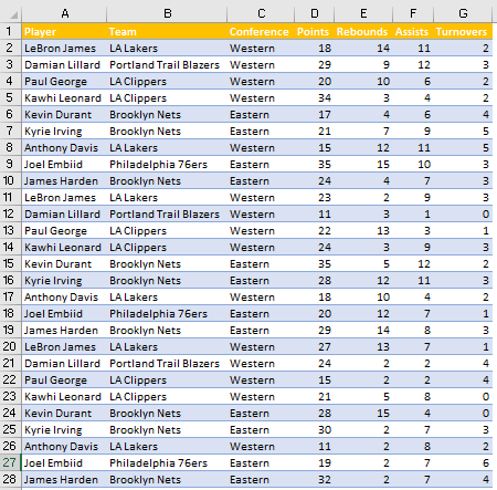
For our example, we will use a list of NBA players with the statistical data from several nights: points, rebounds, assists, and turnovers:
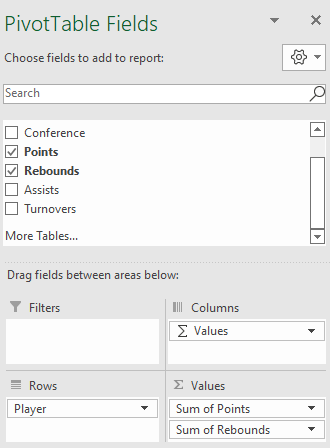
We will insert a Pivot Table by selecting the whole table and then going to Insert tab >> Tables >> PivotTable. We will add points and rebounds to Values Fields (sum of points and sum of rebounds) and Player In Rows Fields:
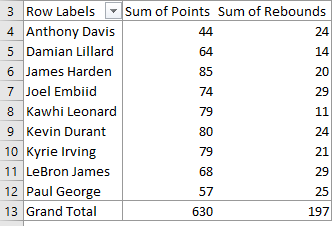
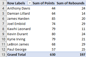
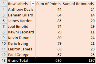
Our table currently looks like this:
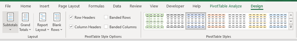
We can add any style and formatting to our table that we want. The easiest way to do so is to select the table and then go to the Design tab. As seen, there are multiple options:
We will first de-select Row and Column Headers, and we will choose a random style from PivotTable Styles. Our table will now look like this:
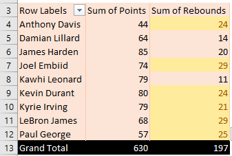
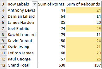
In addition to the Design tab for the Pivot Table, all other formatting options are available. For example, we will define with Conditional Formatting that all numbers in column C (related to players) higher than 20 are highlighted in yellow:
Remove Pivot Table Formatting
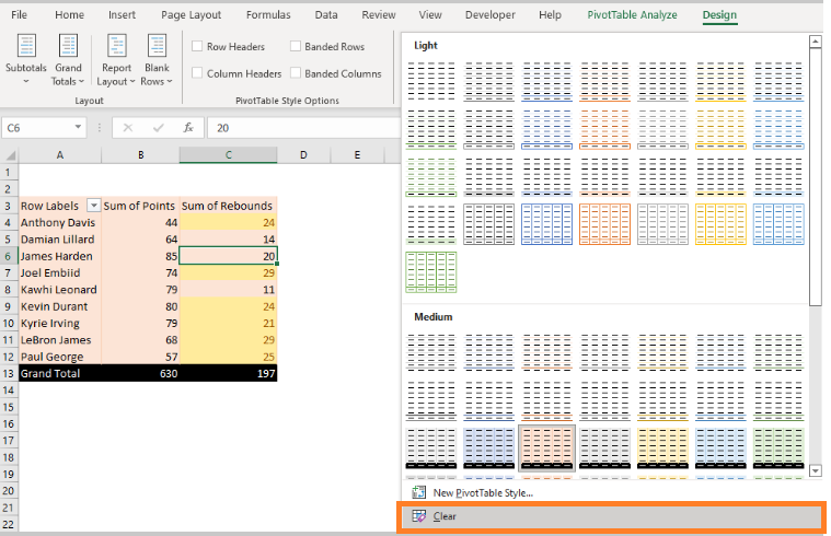
If we set formatting rules for the table through the Design tab, we can easily clear all of the formattings by going to this tab again, and then going to PivotTable Styles and choosing the last option- Clear:
When we click on it, everything that we have set through the Design tab will be erased:
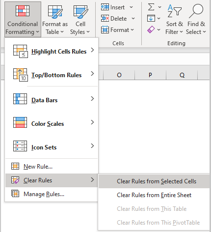
Since we formatted rows in column C through Conditional Formatting, we need to clear this with another option. To do this, we will select the cells that are highlighted in column C, and then go to Home tab >> Conditional Formatting >> Clear Rules >> Clear Rules from Selected Cells:
Our table will be completely blank now: