The biggest change that has ever been done in the Office Suite user interface is the Ribbon. The first release of Excel that uses the Ribbon is Office 2007. It is also present in Office 365.

The idea behind the ribbon is to put there the most important features, so the user will have quick and easy access to them. It is divided into cards, which are divided into groups. Inside each group, there are tools and buttons thematically related to each other.
Hiding the Ribbon
If you need more space in the worksheet, you can increase it by collapsing the ribbon. There are two ways to do this:
1. Click the triangle-shaped button on the right side of the ribbon.
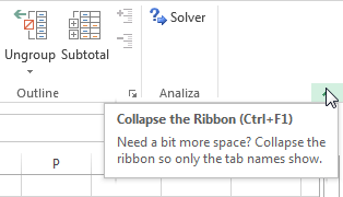
2. Use the Ctrl + F1 keyboard shortcut.
Showing the ribbon
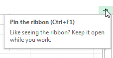
There are two ways to show back the ribbon:
- Use the Ctrl + F1 keyboard shortcut.
- Click one of the tabs.
If you choose the second method you will also have to click the Pin the ribbon button. Otherwise, if you click anywhere outside the ribbon then it will collapse again.
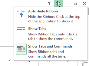
You will find additional options in the upper right corner of the screen, next to the help button.
Ribbon tabs
The ribbon is divided into tabs. In each tab, you can find groups that are related to each other. Each group consists of features and buttons, which are designed for similar tasks. By using them, you can easily access the tool you are interested in, as well as explore other related features.

Excel tabs are divided into the following categories:
FILE
The FILE tab differs from the other tabs. In contrast to other tabs, it has been marked with a different color (for Excel- green). When you click it, it will take you to the Backstage view.
HOME
You will probably spend most of your time in Excel using this tab. It doesn’t contain features that are closely related to each other, but those that are the most popular and handy. Here, among other things you will find: formatting commands, text alignment, cell operations, searching, filtering and sorting data.
INSERT
Select this tab if you need to insert something in the worksheet. It can be a chart, table, picture, etc.
PAGE LAYOUT
This tab contains commands that will help you manipulate the look of your worksheet. Those tools are especially useful when you are planning to print your work.
FORMULAS
All functions that are available in Excel can be found in this tab. They are divided into categories, which you can access by clicking one of the buttons.
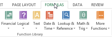
Here, you will also find a number of tools that will help you work with formulas. These tools are formula auditing or defining names.
DATA
With these tools, you can connect to an external data source, such as an SQL database. Tools such as sorting, filtering, and linking options will help you work with very large amounts of data.
REVIEW
This tab contains such tools as check spelling, add comments, translate words and protect worksheets.
VIEW
Here, you can enable or disable various display options. Some of them are also available in the Status bar .
DEVELOPER
This option is hidden by default. To unlock it, go to File >> Options >> Customize Ribbon and click the checkbox. It will add the Developer Tab to the ribbon. Now you will have access to options that can be useful for programmers.
Tool Tabs
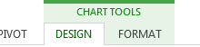
Tool Tabs contain additional tools. They appear right next to the main tabs. Depending on what you are currently working on, you will see different tools. For example, if you work with charts then they will look like this:
Before diving into advanced features, users should solidify their understanding of core tasks like formatting, formulas, and data manipulation. This will enable them to leverage the ribbon’s true potential and unlock Excel’s full potential.
Tomasz Decker
Tool tabs
In addition to cards that are, by default, displayed in the ribbon, there are additional cards that appear when you work with different things.
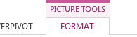
For example, if you work with images, the additional card, called PICTURE TOOLS will appear. It will help you work with images.
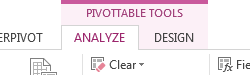
If you create a pivot table, then the PIVOTTABLE TOOLS will appear.
In order to view all available tools using one of the following methods:
- Right-click any field in the ribbon and select Customize the Ribbon.
- Go to FILE >> Options >> Customize Ribbon.
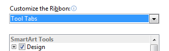
Under Customize the Ribbon, in the upper right corner, you will find a drop-down menu. Click it and select Tool Tabs. After you select this option, below the drop-down menu you will find all Tool Tabs that can be added to the Ribbon. You can expand them and explore their contents.
How to customize the ribbon
The Ribbon is designed to help you achieve greater productivity in Excel. It can be customized to meet your individual needs.
To open the Customize the Ribbon window, do one of the following:
- Go to FILE >> Options >> Customize Ribbon.
- Right-click any field in the ribbon and select Customize Ribbon.
A new window will appear.
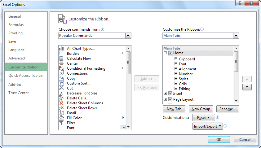
On the right side of the window, you will find items with checkboxes that represent tabs in the ribbon. You can select or deselect them, depending on whether you want the tab to be visible in the ribbon. Expand the tab to see what groups it is composed of. Expand the group to get access to its elements.
Creating a new tab
Another thing you can do with the ribbon (in addition to hiding and displaying its elements), is to create your own tabs. To create a new tab, click the New Tab button.
After you click the box, on the right side you will see a new item, named New Tab (Custom). It includes a group called New Group (Custom).
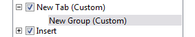
If you want to change the name of the new tab or group, right-click it and choose Rename. Alternatively, you can choose to click the Rename button, which is located below the tabs. In the window that appeared, enter a new name. Notice that when you change the group name, you will have a further opportunity to select the corresponding icon that will be displayed in the tab.
After you change the names of the buttons, Excel leaves the text “(Custom)” at the end of the name. The application does this, so you won’t forget that the tabs have been created by you and are not Excel default tabs.
To add new items, first, click that group, then start adding options and features which you want to be present in the Tab.
Additionally, if you don’t like the position of the tab, you can use the buttons that are located on the right side of the window.
Resetting the ribbon
If you want to go back to the previous settings, click the Reset button. Here, you will find two options.
Reset only the selected ribbon tab
You can use it if you made changes inside one of the default Excel tabs.
Reset all customizations
Undo all changes and restores the ribbon to its original state.
Using the keyboard to work with the Ribbon
If you think that working with Excel with a keyboard is more convenient than with a mouse, you will probably be happy that the individual elements of the ribbon can also be controlled by the keyboard.
If you want to access the ribbon by using the keyboard, press the left Alt keyboard shortcut.
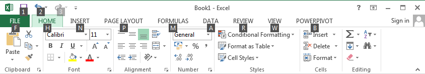
Excel will display icons thanks to which, you know which part of the ribbon corresponds to which character. Here, unlike the keyboard shortcuts, you don’t hold two keys at the same time but press them one after another.
Example:
Suppose that you want to change the font size for the values in the selected cell. The first thing you need to do after pressing the Alt key is to select the Tab you are interested in.
Press the key which is assigned to the tab, even if the tab is currently opened. In our case, press the h button to select the HOME tab. Next, you will get another set of characters. This time, you can select options and features inside the previously selected Tab.
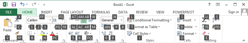
To select the font size, first press “f” and then “s”.
Enter the font size you want and confirm with the Enter key. If you want to return to the previous selection, press the Esc key.
Excel 365 Update
Contextual Ribbon Tabs:
- Excel 365 introduces contextual tabs: These tabs appear temporarily based on the specific task you’re performing. For instance, when working with table, a “Query” tab might pop up alongside the regular tabs, offering relevant formatting options. This can streamline the workflow for specific actions.

- “Tell Me” in Excel 365: This feature acts like a search bar within the ribbon. You can type what you’re looking for (e.g., “Sum cells”), and Excel will direct you to the appropriate tool or function.