One Value Based on Another Cell in Excel

In some cases, you will base the result and formatting of one cell on the result of a different cell on the worksheet.

Take a look at the example below.

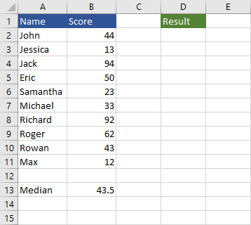
There are 10 people with score results, but only 50% of them will pass.

We are going to pass them, only if their result is better then the median. We are going to display “Pass” or “Fail” in the “Result” table.

This is the formula we are going to use in cell D2.

Make sure that you use absolute reference from cell B13.

Conditional formatting based on the result

The result we display can be further improved, by formatting them with different colors. Here’s how to do it.

Select cells from D2 to D11.

Navigate to Home >> Styles >> Conditional Formatting and choose Manage Rules.

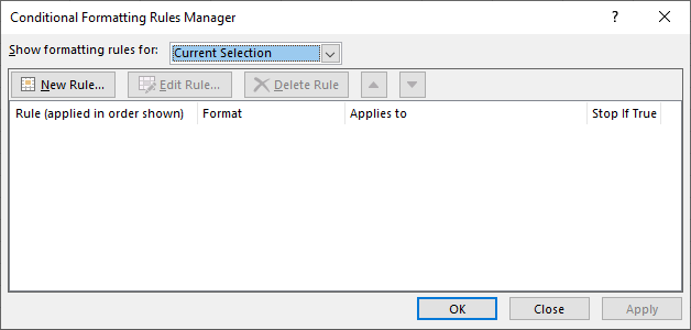
Add the first rule by clicking the New Rule button.

Set the parameters as in the image below.

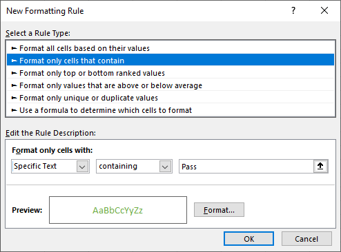
This is the rule for “Pass”.

Create another one, this time for “Fail”. Set the font to red and text to “Fail”.

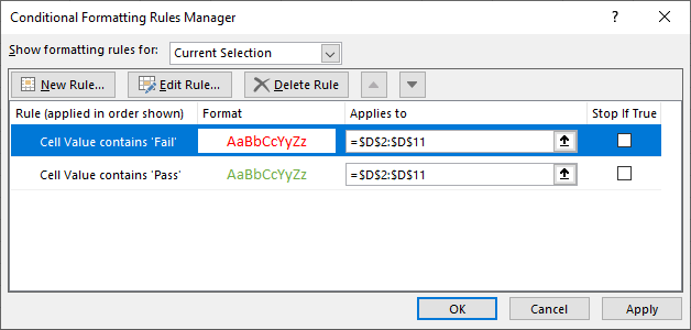
When two rules are created, click OK to apply changes.

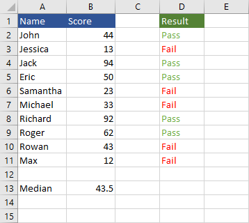
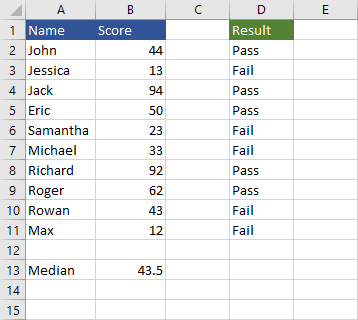
As you can see, half of the students passed the exam, and the other half failed. Thanks to conditional formatting, it looks better now.