The vlookup function is used to look up and retrieve information from the selected column in a table. If you used this function, you probably noticed that the information you retrieved doesn’t keep the original number formatting.
The general formatting cannot be applied by a formula, you have to use VBA code.
First, let’s try to use VLOOKUP and see what happens with the formatting.
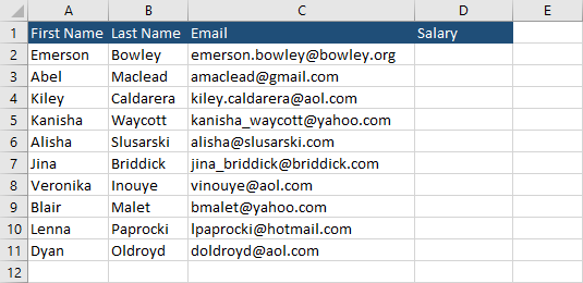
The following worksheet has two sheets.
Sheet1 consists of 10 names in which we want to look up salaries from the other sheet.
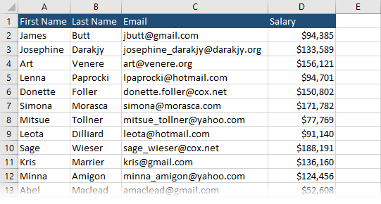
Sheet2 consists of 50 names with salaries and currency formatting. In addition to this, the salary is separated by commas.
Insert the following code into cell D2 in Sheet1.
|
1 |
=VLOOKUP(C2,Sheet2!$C$2:$D$51,2,FALSE) |
Autofill the rest of the cells.
This is the result we get.
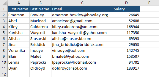
There is no number formatting here. What you get are just raw numbers. In the next part, I’ll show you how you can create the VLOOKUP function that also copies formatting.
Vlookup function with formatting
The following function is similar to the vlookup function. The difference is that this function inserts not only the value but also the source formatting.
Create a new module and insert this code.
|
1 2 3 4 5 6 7 8 9 10 11 |
Function LookupWithFormat(ByRef findValue, ByRef lookupRange As Range, ByRef colRef As Long) Set FindCell = lookupRange.Find(What:=findValue, LookIn:=xlValues) CellAdd = Application.Caller.Address With FindCell myRow = .Row myCol = .Column With .Offset(0, colRef - 1) LookupWithFormat = Format(FindCell.Offset(0, colRef - 1).Value, FindCell.Offset(0, colRef - 1).NumberFormat) End With End With End Function |
Insert the following code into cell E2.
|
1 |
=LookupWithFormat(C2,Sheet2!$C$2:$D$51,2) |
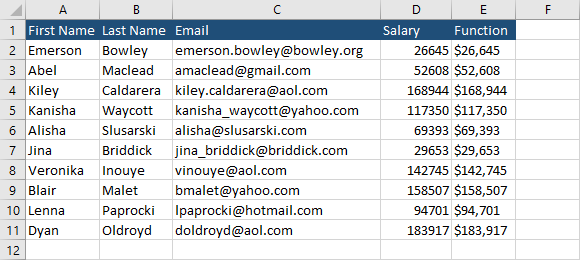
If you run this function, you will get a different result.