Sorting PivotTable is useful, especially when you have to deal with large amounts of data. There are a few ways you can sort your data. You can do it from lowest to highest, from highest to lowest, and in alphabetical order. When you sort your data, it’s much easier to find the values you want.
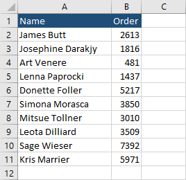
We are going to use the following example to create a PivotTable.
Sort by labels (with arrow button)
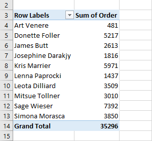
If you create a PivotTable, you will notice that despite the table being unordered, the values in PivotTable are, by default, sorted in alphabetical order from A to Z.
Next, to the Row Labels, there is a little triangle button.
Now, you have two options you can sort the text data: from A to Z and from Z to A.
If you have numbers instead of text, they will sort from smallest to largest or from largest to smallest.
What to remember about sorting data
When you sort data, there are a few things to remember:
- leading spaces will affect sort results. I recommend removing any leading spaces before creating a PivotTable.
- sorting is not case-sensitive.
- you can’t sort by specific type of format, like cell background color, font type, font color, etc.
Sort on a column without an arrow button (by values)
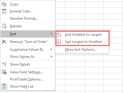
In our example, under the Sum of Order, there is no little triangle button we can click and choose sorting options. In this case, you can right-click inside this row and select Sort. Because the second column deals with numbers, you have two options for sorting: from Smallest to Largest and vice versa.
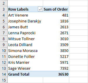
Let’s sort this column from smallest to largest.
Now, as you can see the values inside the second column are displayed in ascending order, and the values in the first column are not.
You can also use the contextual menu for the column, even if there is an AutoSort button.
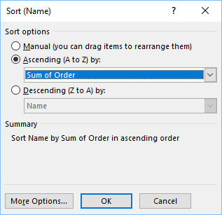
Custom sort PivotTable
If you click the AutoSort button, there is a position called More Sort Options…. Click it to open the Sort window.
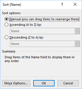
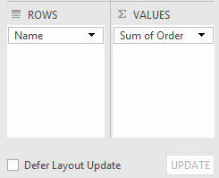
The first position will allow you to manually arrange items by dragging them. Choose this option to sort an individual item. You can’t drag items that are located in the VALUES area. In our case, you can only drag items in the Name column.
Click any cell inside the first column and drag it into a different position.
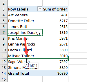
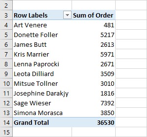
The green line will show you when the item will be placed. Release the cursor to place the item there.
The next two radio buttons are responsible for sorting the first or the second column in ascending or descending fashion.
In the bottom-left corner of the window, there is the More Options… button. Click it for additional options.
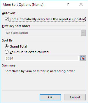
In AutoSort, you can check or uncheck whether you want to sort the PivotTable every time the PivotTable data is updated.
The second option is the First key sort order. This option is available only when the Sort automatically every time the report is updated is unchecked.

There are four default custom orders, the first two for days and the next two for months, you can create your own custom lists.
The last position is Sort By. You can sort by Grand Total or Values in selected column. This option is available if you selected manual sorting in the previous window.
Define custom lists
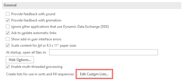
If you want to define your own custom list, navigate to File >> Options and click the Advanced tab.
In the General area, there is a button called Edit Custom Lists….
And there are the 4 custom lists we’ve seen in the More Sort Options window.
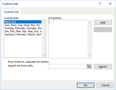
You can’t modify these 4 lists, but you can add your own or edit the ones you already created.
Sort row or column label data using the Ribbon
Another place where you can access sorting options is the Ribbon. Click a cell inside the selected PivotTable column and navigate to Data >> Sort & Filter.
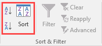
Here, you have three buttons. The two on the left will sort a column in alphabetical order. The big Sort button opens the Sort or Sort By Value windows.